|
|
|
Note to the Reader
Society for Neuroscience. Neuroscience 2002. Presented as a symposium in
Bioinformatics 2002 A Neuroscientist's Guide to Tools and Techniques for
Mining and Refining Massive Data Sets. Organized by Robert W. Williams, PhD.
and Dan Goldowitz, PhD.
Print Friendly
Everyday bioinformatics for neuroscientists: From maps to
microarrays
Robert W. Williams
Center for Neuroscience, Department of Anatomy and Neurobiology,
University of Tennessee, Memphis, Tennessee 38163
Email questions and comments to
rwilliam@nb.utmem.edu
Introduction
This chapter covers two topics:
First, I would like to introduce (or reintroduce) you to some of the key
features of maps of the mouse and human genomes. These maps have become an
important structural substrate around which many types of biological
information is now being assembled. Those of you who have linked recently to
the NCBI, ENSEMBL, and USCS Genome Browser sites for human and mouse genomes
will have encountered the complex graphic conventions and acronyms that are
used to display different types of genetic information. The progress in the
last year has been astonishing and will have an impact on research that is
carried out in most laboratories that have a molecular or genetic research
angle.
My second aim is to summarize some of the basic informatics and
computational tools and tricks used to manage large and small data sets. The
scale of this work can range from a modest stereological analysis of cell
populations in a few dozen cases, to large microarray databases, through to
huge image data sets (see the chapters by P. Thompson and M. Martone). Most
of us now use spreadsheets such as Excel in some capacity to manage lab
data. I hope to show you a few useful tricks for managing large Excel
spreadsheets. But I mainly hope to convince/encourage you that it is easy
and worthwhile to extend beyond disjointed sets of Excel spreadsheets and to
become comfortable, even proficient, using a simple relational database such
as FileMaker or Microsoft Access. Over the past few years our group has
become completely dependent on relational databases. Databases have replaced
notebooks and spreadsheets for most lab work and even for some primary data
analysis. The improvement in lab data handling has been amazing and
initially unrelated files and data set can often be easily merged. Best of
all, our lab data are now accessible using an Internet connection from any
computer in the lab or across the world. Internet databases are obviously
far easier to replicate, archive, and distribute than raw data stuck in a
notebook.
Topic 1: Physical and Genetic Maps
Maps come in two major flavors: physical and genetic. Physical is an odd
word in this context, but signifies that the map is based on sequence data
and on an assemblage of YACs, BACs, and other clonable pieces of chromosomes
that have been ordered into a contiguous stretch of DNA, preferably without
any interruptions or ambiguities. The NCBI site at
www.ncbi.nlm.nih.gov/genome/seq/ NCBIContigInfo.html has a fine description
about how the mouse physical maps (genome sequence) are being assembled.
Quality of these physical maps is now vastly improved over the situation
even one year ago and the progress will continue for several more years.
The unit of measure of a physical map is generally a base pair or nucleotide
(bp or nt). In humans, by convention the 0 bp position is at the telomeric
tip of the short P arm of each chromosome (usually illustrated at the tops
of most figures) and the end is at the tip of the long Q arm. Murine
chromosomes have extremely short P arms (all chromosomes are acrocentric),
and the 0 bp position is within a few megabases (Mb) of the centromere. A
typical chromosome in human or mouse is between 60 and 200 Mb long.
The great majority of genes have now been physically mapped in several key
species (although sometimes they go unrecognized for a while), and the
phrase gene mapping is beginning to loose its original meaning. The focus
now is turning away from mapping genes to mapping phenotypes across sets of
chromosomes and genes. By mapping a phenotype, I actually mean finding the
set of polymorphic genes (genes with multiple alleles) that modulate some
trait, for instance numbers of tyrosine hydroxlyase-positive neurons in the
substantia nigra or risk of developing Alzheimer disease. I’ll come back to
this topic.
In contrast, genetic maps are based on a somewhat more abstract analysis of
the frequency of recombination events that occur during meiosis along
paired-up sister chromosomes. The greater the distance in base pairs or
centimorgans between two points of a single chromosome, the more likely that
a recombination will occur between those two points to break up the original
arrangement of genes on the parental chromosome. That original order is
called the parental haplotype and the order of the recombination is called
the recombinant haplotype.
Until a few years ago, all genetic maps were constructed by computing the
frequency of recombination between genes and markers on chromosomes. The use
of the term genetic in this context seems inappropriate or superfluous, but
the idea was to minimize confusion: genetic maps are sometimes referred to
as meiotic maps, linkage maps, recombination maps, or haplotype maps (that
really helps to minimize confusion!), and the standard unit of measure of a
genetic map is the centimorgan (cM, defined below).
Chromosomes usually measure from 50 to 300 cM.
Box 1: Markers,
SNPs, Microsatellites, QTLs, etc.
In dealing with maps of various types you will need to know
how some key vocabulary is used by most geneticists: What is a marker, a
microsatellite, a SNP, a polygene, a locus, and QTL? A marker is often a
non-functional but polymorphic stretch of DNA, for example a short
microsatellites or a single nucleotide polymorphisms (a SNP).
Microsatellites (a term that derives from hybridization characteristics)
is highly repetitive DNA sequence that tends to be highly polymorphic
because polymerase has a very hard time replicating this boring DNA
accurately. For example the sequence CAGCAGCAGCAGCAG. CAG is a
tri-nucleotide microsatellite repeat that in the right reading frame
will translate into a string of glutamine residues. If a microsatellite
is in an exon, and if the number of repeats is abnormally large, then
bad things can happen to neurons: Huntington disease is an extreme
example. Markers, whether SNPs or microsatellites, will always be useful
for efficiently screening the structure of genomes and the inheritance
of blocks of DNA and blocks of genes. Markers that happen to be within
genes, such as the key microsatellite in the huntingtin gene are of
course interesting in their own right, especially when they correspond
to resistance or susceptibility to a disease.
A polygene is an odd term that refers to the set of polymorphic genes
that collectively control the variation in a trait. For example, the
BRCA1 and BRCA2 genes are part of a cancer susceptibility polygene.
Usually, we do not know the membership of a polygene; we just know that
a small or large number of scattered genes modulate some trait. Finally,
what is a locus? This is a term used to hedge bets. We would like to
call everything a gene, but many times we only know the approximate
chromosomal position that appears to contain factors that modulate
variation in a trait. This chromosomal region may contain a single
causative gene or it may contain a cluster of genes that collectively
modulate a trait. The safe term is locus. A QTL is a so-called
quantitative trait locus. That translates as follows: a chromosomal
region that harbors one or more polymorphic genes that influence the
variation in a trait in a graded (quantitative) manner. QTLs are
relatives of the modifier loci that one sometimes hears about in the
context of major disease genes and knockouts. A modifier locus is
usually a QTL that modulates the severity of a phenotype. |
The frequency of
recombination is variable and depends on the chromosome, the species or
strains, and the sex. Genetic maps are elastic. Genes and markers on genetic
maps have the same order, but distances vary among experiments and
populations. A useful metaphor: Genetic maps are similar to maps that
measure the separation between cities in terms of the standard driving times
required to get from one to another. Those times will be very contingent. In
contrast, a physical map is structural and not subject to much change.
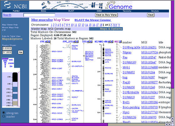
Let’s look at the type of maps that are now available on line at NCBI.
Reading from the left side of this figure 2, we first see a cytogenetic
ideogram of the smallest of the mice chromosomes, Chr 19. The Zoom is at its
lowest setting and the lines and columns to the right side cover most of Chr
19. The left-most line is the approximate distance in millions of base pairs
(M in the figure) from the tip of the chromosome; the right-most line is the
genetic map measured in centimorgans. Again, there is no single genetic map,
but many alternatives, and the alternative that is displayed by NCBI is the
Mouse Genome Informatics group’s consensus map. There are lots of acronyms
of these and other maps (FPC for finger print clone), and you can find out
what each line or trace means by clicking on the column headers.
Will genetic maps fade out into the history of science as physical maps get
better and better? Absolutely not. The simple reason is that when we try to
discover the genetic basis of differences in phenotype, we almost invariable
rely on recombination events to test the likelihood that a sequence variant
is associated with a variant phenotype. (Cytogenetic abnormalities are an
important exception.) Most of the discoveries of genes and gene
polymorphisms (alleles) associated with diseases rely on probabilistic
recombination events—either the historical recombinations between
populations or the more recent recombination that are unique to large and
small families. Even if we could snap our fingers and sequence the entire
genome of every one on earth, we would still end up tracking the sites of
recombinations and their relations with variation in phenotypes.
Mapping Genes
Almost any sequence of nucleotides from Drosophila, C. elegans, human, and
mouse can now be physically mapped using BLAT or BLAST to the nearest base
pair in a matter of seconds (see Effective Mining of Information in Sequence
Databases, by David Deitcher in this Short Course). Jim Kent’s BLAT program
illustrated below is a remarkable web tool that works well for mouse and
human sequence. Paste any nucleotide or peptide sequence into BLAT at
genome.ucsc.edu/cgi-bin/hgGateway?db=hg12 and within 1–2 seconds you will be
rewarded with a list of hits. This new resource made it possible in
collaboration with John Hogenesch and colleagues at the Genome Institute of the Novartis Foundation,
to locate the base pair position of almost all the GenBank entries used to
make the Affymetrix U74Av2 GeneChip (Fig. 5).
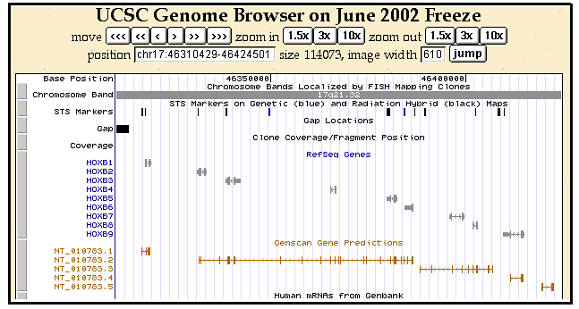
If you simply need to explore a genome location to view sequence,
intron-exon structure, fish out promoter motifs, then just enter a key word
and the BLAT search will deliver you to a particular part of the genome. In
the figure below, I entered a search for HOXB8. Then zoomed-out to get a
view of the entire human HOXB complex on Chr.

Figure 1. Physical and genetic maps of mouse chromosome 19 from the
National Center for Bioinformatics. This figure can be expanded to reveal
fine details and sequence from almost any region.
If you visit this impressive web site you can get complete descriptions of
the various traces that are essentially graphical annotations and summaries
of the human and mouse genomes. You can zoom into the level of the
nucleotide sequence.
Mapping Brain and Behavioral Traits
Mapping phenotypes is a much more difficult task these days than locating an
arbitrary gene sequence. When we talk about mapping a gene that influences
circadian rhythm, neuron number, anxiety, susceptibility to Parkinson
disease, alcoholism, or schizophrenia, we are really talking about matching
differences in structure or function to one or more chromosomal regions;
so-called gene loci (see BOX 1). We would love to map genes for Parkinson
disease, but what that usually means is that we would like to identify
statistically significant association between variability in susceptibility
to Parkinson disease with a genetic polymorphism (variation) that may be
distributed widely across the genome. In other words, we are mapping a
phenotype to multiple regions of the genome. This is the crux of forward
genetics. If the process of mapping these traits intrigues you, then link to
a previous Short Course tutorial on forward genetic methods at
www.nervenet.org/papers/shortsourse98.html.
This Short Course contains much additional information on procedures for
mapping traits and genes.
Chromosome maps have a complex and heterogeneous structure. This is visible
at the cytogenetic level as differences in banding patterns and at a finer
grain as large fluctuations in mean gene density. The haphazard way in which
chromosomes differ between even fairly closely related species demonstrates
abundant chromosomal plasticity. However, gene location, order, and
orientation can also be important as highlighted by the conservation of the
HOXB gene families illustrated in figure 2 from the extremely useful Genome
Brower web site at the University of California Santa Cruz.

Figure 2. Detailed view of the human HOXB complex on chromosome 17
taken from the University of California Santa Cruz Genome Browser.
Topic 2: Excel and relational databases
Bioinformatics is closely associated with genomics and the analysis of
sequence data and maps (see Box 2), but in this section I would like to
broaden that definition to include handling information that is typically
generated and processed in laboratories every day. In the biotech and
pharmaceutical industry work of this type is handled by a LIM system (a
laboratory information management system). This type of everyday
“bioinformatics” often starts with simple decisions about unique case Ids
and identifiers to be used in experiments, extends through to the
organization, use, and security of lab notebooks, and often ends with the
extraction, analysis and archiving of data and experiments with spreadsheets
and statistical programs. Most of this type of information handling is taken
for granted and many of us (and especially our mentors) assume that there is
not much room for modification or improvement in the daily cycle of data
generation, analysis, and publication.
In fact, the efficiency and sophistication of the day-to-day aspects of data
acquisition and handling can be substantially improved. It is becoming more
important to have a lab database and a web site for more that just a
curriculum vitae and a set of pdf files. Lab web sites are becoming one of
the most effective ways to communicate results. www.nervenet.org provides a
good example of how our lab publishes data on-line.
In this section I will make some suggestions about how to move in the
direction of using relational databases to improve lab informatics. The
expense of entering this new sphere is modest and the gain in scientific
efficiency can be substantial. Best of all, these new tools make
collaborative research across cities and continents much more practical.
Excel: uses and abuses
Exposure to practical lab bioinformatics often starts with Excel. Excel has
become a pervasive (almost obligatory) vehicle for data email exchange. It
is also a very powerful tool for analysis. Not many of us have read or
reread the Excel manual: we usually learn on the fly. Let me summarize some
of the key features:
1. File size. Excel has a limit of 65,536 rows and 256 columns. That
is usually not a problem. Our lab still uses Excel for some aspects of
microarray analysis. You can easily pack 12,500 rows and 240 columns worth
of data into an Excel file and you can have multiple spreadsheets in a
single file. We have several Excel files that are about 120 MB in size, and
the program runs reliably if given 300 MB of memory. However, for all but
the smallest projects, it is not a good idea to store data files long term
in Excel. You will hear more about this in the next section. In brief, Excel
is for analysis—not for archiving and databasing. Running up against the
table size limits of Excel is not hard these days. If you begin to work with
even a single Affymetrix GeneChip at the cell level (about 500,000
cells/chip) then you will have to use another software tool (SAS, Systat,
SPSS, S-Plus, Matlab, DataDesk, FileMaker, MySQL, PosgreSQL, etc). More on
this later in the section on Relational Databases.
2. Transposing data. It is easy to transpose a data set in Excel
(that is, switch rows to columns and columns to rows). Select the region of
interest and copy it. Then select the upper left cell of the destination for
the transposed data and use the Paste Special command. There is a check box
labeled “transpose.” Paste Special is a very useful feature that we use
extensively to convert equations to values. This can reduce RAM requirements
and speed execution. Keep equations if you need them permanently for
updating. But if you just want the values, convert equations to values using
Paste Special. You can also transpose values and leave formats alone.

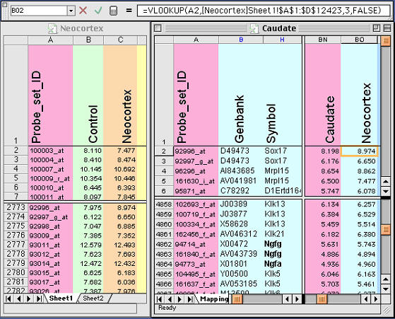
Figure 3. Using lookup functions in Excel to exchange selected
data from between files. Details of this method are described in the text.
Note the equation at the top of this figure. This equation places new data
from the Neocortex database (left side) into the Neocortex column of the
Caudate database (right side)
3. Merging complex tables that share a unique field is easy to do in
Excel. Let’s say you have an Excel table consisting of 6,000 gene
transcripts expressed in the caudate nucleus. You have another list of
12,000 gene transcripts with data on neocortex expression sent to you by a
colleague. You want to extract the neocortical values and align them with
the set of 6000 caudate transcript values. The problem is that the tables do
not overlap perfectly. The solution is simple. If the two tables share a
common field type, for example an Affymetrix ID number or a GenBank
accession number, you are in business. Just use the vertical lookup command
as shown in Fig. 3. Excel will help explain the use, but here is my version
of help: open both files, then add a new column in the Caudate Table labeled
Neocortex. Type in a variant of the equation that is listed toward the top
of the next figure. These equations have the form: =VLOOKUP(CellID,
LookupTable, Offset, FALSE)
.The CellID (A2 in the example below) is the spreadsheet cell that contains
the unique ID that both tables share (the Probe set ID 92996_at in this
example). The Neocortex table is just a region that will be interrogated by
Excel to find the single matching row in the Neocortex table (row 2773 in
the figure); the Offset is an integer that instructs Excel to copy data from
the Nth column to the right of the ID column. In this case, the offset is 3.
FALSE is a flag that instructs Excel to use only perfect matches. Make sure
that this equation works for the first few cells in your new column and then
copy the formula down the whole column. You may need to put dollar signs in
front of some cell references to lock the reference in place so that the
definition of the table does not change as you copy down the column.
4. Excel as a statistical analysis program. Simple statistics (mean,
median, average, errors) can be computed quickly for thousands of rows or
columns of data in Excel. This is an ideal use of Excel. It is also possible
to perform tens of thousands of t tests in Excel in less than a minute. If
you have ten arrays worth of data (5 wildtype and 5 knockout array data
sets), then you can perform a quick t test for every transcript using the
formula:
=TTEST(WT1:WT5; KO1:KO5, 2, 3)
WT1:WT5 is the range of the wildtype data in a single row (five columns
worth of values. KO1:KO5 is the same thing for knockout samples. The
parameter 2 instructs Excel to compute the 2-tailed probability. The final
parameter 3 instructs Excel to assume that the variance of the two groups is
not equal. Excel will return the probability of the t test rather than the t
value. If you have done any array work you will already be familiar with the
multiple tests problem (see the chapter in this Short Course by Dan
Geschwind and colleagues). An array consisting of 10,000 transcripts should
generate about 500 false positive results with alpha probabilities of less
than 0.05; 100 with P <.01; and 10 with a P <.001, etc. If you plot the P
values against their rank order (rank on the x axis from lowest to highest P
values, and the actual P value or log of the P value on the Y axis), then
you will end up with an interesting plot that can be helpful to estimate how
many false discoveries you are making at any given P value. (For more on the
Benjamini and Hochberg method of false discovery rates see
www.math.tau.ac.il/~roee/index.htm ).
It is not a good idea to use Excel in place of sophisticated statistics
programs. If you are gearing up for regression analysis, ANOVA,
non-parametric statistics, factor analysis, principal component analysis,
then buy one of the many good statistics packages. SAS, SPSS, StatView,
Matlab, and DataDesk are powerful tools. DataDesk in particular is an
amazing program that makes working with very large data sets more like a
game than a chore. We routinely review all of our array data with DataDesk
and use this program to generate draft figures for papers. If you buy this
inexpensive program be sure to work through the excellent manual. Ample
rewards.
5. Excel to normalize array data sets. This is a good use for Excel.
Excel can compute rank orders: =RANK(TEST_CELL, ALL_CELLS); compute the
logarithm base 2: =LOG(VALUE, 2); and compute the Z-score for a cell: =STANDARIZE(VALUE,AVERAGE,
STDEV). In many of these formulas you will need to lock one cell reference
so that values do not change when you copy or fill. Use the dollar sign to
lock a reference in a formula, for example if the cell that contains the
average is C12450, then enter it as C$12450. If you copy down the column
then the reference to the average will not change. If you copy to the right
however, then the reference may change to D$12450, since the column letter
was not locked. To lock both use the format $C$12450.
6. Using Excel as a database program. Don’t bother. Excel is great,
but it is definitely not a database program. If you have played with the
database functions that are built into Excel then you have all of the
experience and motivation that you need to graduate to one of several much
better, more powerful, and easier to use database

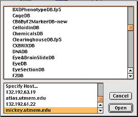
Figure 4.
Internet access to over 50 laboratory databases hosted on
an inexpensive but robust lab computer: a Macintosh G4 running OS X and
FileMaker server. The top panel is a partal listing of some of the
related databases, including CageDB (animal colony), CelloidinDB
(histology), EyeDB (eye phenotypes), DNADB (sample preparation), F2DB
(genotypes), etc. |
programs. FileMaker Pro and Access are programs with which you can get
comfortable in a few days. Read the next section for details on the
migration to relational databases.
Moving beyond Excel: Relational databases
A bioinformatic imbalance. We often do a great job handling the hard
problems in neuroscience and bioinformatics but often neglect to take care
of the simple housekeeping. This imbalance can lead to serious problems.
Imagine a sophisticated research lab performing hundreds of microarray
experiments and generating and processing megabytes of data every day. Such
a lab will almost invariably have expensive bioinformatics tools (GeneSpring,
SpotFire, etc.) and computer systems for handling array data. But the same
lab may not have a simple database to track the large number of tissue and
RNA samples that are stored in several freezers. In order to confirm the sex
and age of all of the cases in the array data base they may have to rummage
through a set of lab note books and Excel spreadsheets. To determine the
size of the litter to which a particular animal belonged may involve the
laborious analysis of animal cage cards kept in a shoebox in the animal
colony. It may not be practical to determine even after an interval of a few
months which of several investigators, students, or technicians extracted
the RNA; did they use Trizol or RNAStat?
These examples highlight a problem in the typical application of
bioinformatics. We tend to think of bioinformatics as high level analysis
that is applied at the final stages of preparing papers for publication. The
bioinformatic tools enter ex machina to the rescue. Most of us run
microarrays and then learn how to apply sophisticated statistical methods to
parse and interpret patterns of gene expression change. Bioinformatics
should actually be built into a laboratory from the ground up. Data should
ideally flow from one stage and level to the next without the need to
transcribe or reformat. Below is one example that describes how to
accomplish this transformation in your laboratory information management.
The limits of spreadsheets. In 1994 we began a series of experiments
with the aim of estimating the population of retinal ganglion cell axons in
the optic nerves of several hundred (now over a thousand) mice. For each
optic nerve we typically counted 25 electron micrographs and entered the
counts per micrographs and per case in a single row of an Excel spreadsheet.
We calculated means and standard errors for each nerve and row of data.
There seems to be no significant downside to this simple system.
There were a few minor problems that in aggregate became serious and that
illustrated the inadequacy of using Excel as a research database. How does
one handle right and left optic nerves when both sides are counted? That
seems simple; just enter the two sides in separate rows. The consequence is
that some animals were represented on two rows, whereas the majority are
represented on one row.
A second problem was that every time we added data for a particular strain
we had to rewrite some of the Excel formulas used to compute strain
averages. It became awkward to maintain both individual data and strain
averages in a single spreadsheet.
A third problem was keeping track of the latest version of the spreadsheet.
As many as three investigators were working on the spreadsheet each day, and
it was difficult to track versions and to make sure that information was
accumulated and collated correctly. This was a pain to do especially after
the Excel file grew to a large size.
A fourth problem involved the integration of other data types into the
spreadsheet. When we were writing up our results it became obvious that we
would need to consider variables such as brain weight, age, sex, body
weight, and litter size as potential modulators of retinal ganglion cell
axon number. Unfortunately, these data types were scattered in several other
databases. We diligently transcribed data from cage cards and other small
Excel databases and lab notebooks into our optic nerve spreadsheet. This
transcription was associated with the introduction of many transcription
errors and every new case that we added required us to transcribe data from
2–4 other notebooks.
Box 2: Good reading and reference.
Biological sequence analysis: probabilistic models of proteins and
nucleic acids (1998) by R Durbin, SR Eddy, A Krogh, G. Mitchison. $35.
The standard text on sequence analysis; the core topic of
bioinformatics. You can take a tour of the first 23 pages of this book
at Amazon.com.
Bioinformatics, a practical guide to the analysis of genes and proteins
2nd ed. (2001) edited by AD Baxevanis, BF Francis Ouellette. $70.
Provides an overview of common resources and an introduction to Perl.
The main drawback is that practical web-based bioinformatics is moving
so quickly that revisions are needed quarterly. A careful reading of
NCBI on-line documentation will cover much of the same ground. But if
you need hardcopy for bedtime reading...
Bioinformatics, the machine learning approach 2nd ed. (2001) by P Baldi,
S Brunak. $50. A more conceptual companion to the Practical Guide. Most
of the Amazon.com reviews are favorable, but I have to agree that the
coverage of topics I know best (array analysis) is of uneven quality.
Chapter 13 includes an armada of web resources for molecular
bioinformatics that is still useful.
Biometry, 3rd ed. (2001) by RR Sokal, FJ Rohlf. $96. This is one of the
best first courses you can take in statistics. Full of fine examples.
Were you aware that the standard deviation is a biased estimate and is
usually too low (p. 53)? This book does not have statistical tables.
Data reduction and error analysis for the physical sciences. 2nd ed.
(1992) by PR Bevington, DK Robinson. $50. Predates bioinformatics but if
you want an absolutely lucid presentation of the foundations of data
analysis with lots of practical advice and code snippets this is the
right Short Course. Includes some of the statistical tables missing from
Biometry.
Applied Multivariate Statistical Analysis, 5th ed (1998) RA Johnson, DW
Wichern. $105. This volume is a classic but rigorous coverage (“more
equation than words”) that covers the mind-bending world of multivariate
analysis. SK Kachigan wrote a much more accessible and shorter text:
($30, Multivariate Statistical Analysis: A Conceptual Introduction). LG
Grimm and R Yarnold assembled a collection of solid and accessible
chapters in Reading and Understanding Multivariate Statistics ($21) that
gets strong reviews on Amazon.
Fundamentals of database systems 3rd ed (200) by R Elmasri, SB Navathe.
$70. A thorough textbook that will introduce you to the theory and
practice of implementing database systems. |
The solution. The solution was obvious but seemed both risky and
impractical: convert our entire laboratory to a relational database
management system and begin to enter and reenter all data into a set of
interconnected database files or tables. The idea was to eliminate
laboratory notebooks and spreadsheets as much as possible. The process began
in the animal colony and extended through to post publication databases that
are now on-line.
What is a relation? The key feature of a relational database is that
it consists of an often large number of small tables of data that are linked
using key ID fields (for example the Probe_set_ID field in the previous
example).
Instead of trying to cram all data types into a single unwieldy table (the
Excel model), the idea is to parse data into more manageable and logical
pieces. The structure or scheme of a whole lab database system is then
defined in large part by how information flows between and among the various
tables. In the context of an animal colony, rather than having a single
complex ColonyDB table, it is related tables: CageDB, a RackDB, an AnimalDB,
more effective to break up the data types into four smaller LitterDB. These
four tables would all be linked by relations and key fields. For example,
each cage in the CageDB has a Rack_ID. The relation provides a conduit for
information flow and display. A very important idea in relational databases
design is to minimize redundant data among the related tables. Ideally, all
data only are entered into the single most appropriate table. You do not
want to have to enter the sex and age of an animal more than once. A perhaps
counterintuitive example: birth data would typically be entered into the
LitterDB, not the AnimalDB. The AnimalDB would inherit the date of birth
data by following the relational trail between a specific animal and the
litter to which it belongs. Minimizing data redundancy actually improves the
data integrity of the system. You won’t end up with animals that have two or
more different dates of birth. The organization of your database and how you
view and work with the data are two separate issues. Don’t confuse the
underlying database structure with the database interface. For example, the
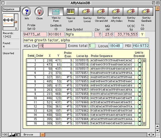
form illustrated in Fig 5, actually displays data from four different tables
and makes use of relations that rely on the Probe Set ID, the Gene Symbol,
the Locus Link ID, and the GenBank accession number. The layout of the form
can be changed in a matter of seconds to simplify data entry or viewing.
Once the right relations have been made it is also simple to compute new
values and new field types based on data in a multitude of different tables.
You can export and print data from any and all of the tables, and you can
compute new data types across the tables.

Figure 5. Example of a one-to-many relation being used to track
and analyze microarray data. The primary database table contains 12,422
records, each of which corresponds to a unique Probe Set ID (94733_at in
this case). Each probe set, in turn, relates to 16 perfect matches held as
individual records in a second lower-level database table-- the Probe
Sequences that are shown in the lower panel. Selecting the Link to Ensembl
button (right side) opens a window on the www.Ensembl.org mouse sequence web
site. Apparently complex databases of this type are simple to make using
FileMaker.
Choosing a database is a important issue since you will probably
have to live with, manage, and pay for occasional upgrades of software for a
long time. The choice is not irrevocable, but migrating from one database to
another can take months. Even a “simple” upgrade can take weeks.
We considered and experimented with a few alternative relational database
programs, including Microsoft’s Access, FileMaker Pro, Helix, Acius’s 4D,
and Panorama. FileMaker was our final choice because of the ease of
implementing complex and visually self-explanatory tables and relations. It
lacks many sophisticated features expected on enterprise products like
Oracle 9, but that is not what we needed. FileMaker now has strong support
for Macintosh, Windows, and Linux platforms. Upgrades have kept pace with
technology without sacrificing ease of implementation. The interface with
Excel is also smooth, making FileMaker an easy upgrade to a relational
database system.
FileMaker vs. MySQL. We have compared the efficiency of implementing
database systems in FileMaker and a free and powerful relational database
called MySQL (Fig. 6). The Mouse Brain Library (www.mbl.org) was originally
implemented as a FileMaker database in just under two weeks by a high school
senior with strong programming skills. This web-accessible database has
performed admirably for several years with almost no unintentional downtime
and now accommodates a wide variety of images for approximately 3000
histological slides and over 200 strains of mice. The Internet interface was
not difficult to implement in FileMaker and allows rapid searches by
genotype for acquisition of images.


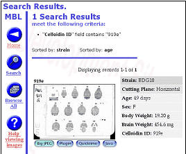
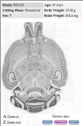
Figure 6. Internet implementations of the Mouse Brain Library (www.mbl.org)
using FileMaker or MySQL The MBL in concert with the iScope, and a
collection of C++ and CGI-like web interface programs deliver images
that range in resolution from whole slides (top), down to ~0.2 microns
per pixel per slide. The iScope is an Internet-driven microscope that
can deliver Z-axis image stacks in color and at sizes up to 1280x960
pixels. These stacks are suitable for high-resolution on-line
high-resolution stereology. |
Once we had built and full tested the FileMaker version we then decided to
replicate the entire system using a free and powerful relational database
called MySQL on a Linux platform. This free implementation took a skilled
database programmer just over 3 months. That is not atypical for MySQL.
However, replicating the MySQL implementation from one site to another site
took less than a week. The moral is that if you want to maximize efficiency
of time and ease of implementation then use a database system that has a
strong and logical interface and high-level graphical interface tools. In
contrast, if you want to provide a free system for use by a broader
community then either convert to MySQL or PostgreSQL (both open source
databases that run on most major operating systems: see www.mysql.com and
www.us.postgresql.org). If speed is a major consideration (lots of array
files), then MySQL is now a faster database management system than
PostgreSQL or FileMaker. For a cogent comparison of these DBMS see
www.webtechniques.com/archives/2001/09/jepson/.
A precaution: There is a certain macho urge to use the most robust
heavy-iron commercial program you can get your hands on as part of a
laboratory database system. Oracle, Sybase, and similar high-end systems are
intended primarily for mission-critical 24:7 activity (student records,
payroll, etc.). Experts on databases generally know these systems well, and
they genuinely think they are being helpful by recommending Oracle with its
sophisticated transactional processing. But Oracle and Sybase are a mismatch
for a typical laboratory. Research and lab databases need to change on a
weekly basis. The layout of fields for data entry may change on a daily
basis. Local control, speed, and mobility are far more important than
processing speed or high level feature sets. Don’t go hunting with a tank.
You need to know how to make changes to the structure of your tables, in the
layout of your entry forms, and how to efficiently export data for
downstream statistical analysis. A strong point in favor of Excel is its
transparency, and you don’t want to lose that advantage when moving to a
relational database. You need to retain full control of your own data.
Security. Backing up and making weekly permanent archives are both
critical. The difference between a backup and an archive is that the backup
is volatile on a daily, weekly, or monthly basis and will be overwritten at
some point. In contrast, archives are intended to be as permanent as
possible. Even the simple systems such as FileMaker Server Edition will
backup on any schedule you would like. Archiving to CD or DVD at the end of
the week is a new obligation that needs to be taken seriously, but that
would be true no matter what system you use.

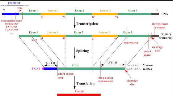
Figure 7. Gene to protein synopsis taken from the Google image
archive (source: Rockefeller Univ.)
Acknowledgments
This work was supported in part by grants from the Human Brain Project (MH
62009). I thank my colleagues Drs. Lu Lu, David Airey, Glenn Rosen, Mel
Park, Guomin Zhou, Elissa Chesler, Siming Shou, Ken Manly, and Jonathan
Nissanov. Special thanks to an extraordinary group of programmers: Tony
Capra, Michael Connolly, Alex Williams, Nathan Laporte, Arthur Centeno, and
Yanhua Qu. Thanks to Emily Carps for help editing.
Williams RW (2002) Everyday bioinformatics for neuroscientists: from maps to
microarays. In: Bioinformatics 2002: a neuroscientist’s guide to tools and
techniques for mining and refining massive data sets. (Williams RW,
Goldowitz D, eds) pp. XX–XX. Washington: Society for Neuroscience.
Copyright © 2002 by R.W. Williams
|
|
|

 Publications