 |
| |||||
|
| ||||||||
|
| ||||||||
Home  Publications Publications |
|
|
Note to the Reader This is a revised edition of a review published in Mouse Brain Development (Springer, ISBN 3540666648, $169 from Amazon.com). Text additions and modification are in brackets. [...]. Williams RW (2000) Mapping genes that modulate brain development: a quantitative genetic approach. In: Mouse brain development (Goffinet AF, Rakic P, eds). Springer Verlag, New York, pp 21–49.
Print Friendly Contents 1. Why brain weight and neuron number matter
In my opinion there are only quantitative differences, not qualitative differences, between the brain of a man and that of a mouse. Ramón y Cajal (1890)
The difference in behavioral capacity between man and chimpanzee may be no more than the addition of one cell generation in the segmentation of the neuroblasts which form the cerebral network. Lashley (1949)
IntroductionThe complexity of CNS development is staggering. In mice a total of
approximately 75 million neurons and 25 million glial cells are generated,
moved, connected, and integrated into hundreds of different circuits over
a period of one month. The process is coordinated by the expression of a
large fraction of the genome—as many as 40,000 genes may be involved
(Sutcliffe 1988; Adams et al. 1993). These same genes coordinate the
development of the human brain, but a thousand times more neurons are
generated (Williams and Herrup 1988) and their integration and training
take more than a decade. While 5,000 of these genes have common roles in
cellular metabolism, this still leaves a huge complement that have
selective, transient, and partially redundant roles in the development of
different parts of the brain (Usui et al. 1994; Gautvik et al. 1996).
Reductionist approaches that focus on isolated processes and molecules may
seem hopelessly inadequate, but they are an absolute necessity at this
early stage of analysis and understanding. Why brain weight and neuron number matter Metabolic constraints. There are several reasons why differences in brain size and neuron number are interesting and biologically significant. First, relative to its size, the brain with its large population of neurons consumes a disproportionate amount of energy (Clark 1994). The high cost of making, training, and maintaining this metabolically demanding organ has wide-ranging effects on an animal's development and behavior (Sacher and Staffeldt 1974; Eisenberg and Wilson 1978; Martin, 1981; Armstrong 1983; Hofman, 1983; Pagel and Harvey 1990; Allman et al. 1993). Humans are an extreme example, with a brain that is 10 times heavier than expected on the basis of body weight. We afford this luxury by developing slowly and by having an efficient diet (Aiello and Wheeler 1995). Given the fact that we are such a large-brained species, it may be a surprise to learn that mice have brains that are proportionally just as large as those of humans. A 22-gm adult mouse typically has a 450-mg brain, whereas a 66-kg human typically has a 1350-gm brain, 2% in both cases. Functional correlates. A second and almost self-evident reason to be interested in brain weight and neuron number is that variation in these simple parameters is associated with variation in behavior (Lashley 1949; Rensch 1956; Wimer and Prater 1966; Fuller and Herman 1972; Roderick et al. 1979; Fuller, 1979; Crusio et al. 1989; Jacobs et al. 1990; Belknap et al. 1992; Aboitiz 1996; Keverne et al. 1996). This is most clear-cut when specific regions of the brains of different species or individuals are compared. For example, in song birds the volume of song system nuclei and numbers of neurons tend to be positively correlated with different features of song production (e.g., DeVoogd et al. 1993; Ward et al. 1998). Another fine example—although strongly negative in this case—is the correlation in mice between avoidance learning and the size of the infrapyramidal projection from dentate gyrus to CA3 (Schwegler and Lipp 1983; Lipp et al. 1989). Insights into CNS development. My colleagues
and I are interested in brain weight and neuron number for a third reason:
as a means to map, clone, and characterize genes that control the
proliferation, differentiation, and death of cells in the CNS (Williams
and Herrup
1988; Williams et al.
1998a). These genes are entry points into molecular networks that
control brain development. Differences in brain weight are proportional to
total brain DNA content and consequently to total CNS cell numbers (Zamenhof
and von Marthens 1976). This is true even in neonatal mice, before
appreciable glial cell production (Zamenhof et al. 1971; Zamenhof and von
Marthens 1976). For this reason, brain weight is a surprisingly good
surrogate measure for total cell number in mice, as in humans (Pakkenberg
and Gundersen 1996).
The biometric analysis of the size and structure of the mouse CNS Precedents. In the late 1960s, Thomas Roderick, John Fuller, Douglas Wahlsten, and Richard and Cynthia Wimer began an ambitious program to manipulate neuroanatomical traits in mice by selective breeding (Roderick 1976). Their aim was to explore correlated changes in behavior. They gave the rapidly expanding field of behavioral neurogenetics a rigorous foundation in quantitative and statistical neuroanatomy (Wimer et al. 1969; Fuller and Geils 1972; Wahlsten 1975; Roderick et al. 1976; Fuller 1979; Wimer 1979; Wimer and Wimer 1985). Rather than relying on mutants, they exploited the substantial variation among standard inbred strains of mice. This work led to some important breakthroughs and some brick walls. One of the breakthroughs was successfully selecting for substantial differences in brain weight over less than 20 generations (Fuller 1979). An obvious limitation, highlighted by Roderick (1976), was that it was not possible to map gene loci responsible for the remarkable quantitative variation in CNS size, regional architecture, or behavior. A new opportunity. The situation has
changed radically in the past decade (Lander and Botstein 1989; Plomin et
al. 1991; Johnson et al. 1992; Belknap et al. 1992; Tanksley 1993; Frankel
1995; Crawley et al., 1997). Computational methods and molecular
reagents—particularly the polymerase chain reaction method—have become so
powerful and economical that it is now practical to systematically dissect
complex polygenic traits such as brain weight into sets of single
well-defined QTLs. Virtually any heritable trait in mice, whether
structural, physiological, pharmacological, or behavioral, can be targeted
for analysis. Recent examples in mice include epilepsy (Rise et al.,
1991), effects of ethanol and haloperidol (Plomin et al. 1993; Belknap et
al. 1993; Hitzemann et al. 1994; Kanes et al. 1996; Buck et al. 1997);
patterns of sleep and activity (Toth and Williams, 1998), and the mouse
equivalent of anxiety (Flint et al. 1995). As illustrated in the work of
Belknap and colleagues (1992), it is now feasible to continue the
systematic genetic dissection of the mouse CNS begun in the late 1960s and
to start identifying genes that underlie heritable variation in CNS size
and structure. Brain weight is highly variable. Brain weight is highly variable among strains reared in a common environment. For example, both A/J and DBA/2J have average brain weights close to 410 mg, whereas C57BL/6J and BALB/cJ have weights close to 510 mg. The variation within each strain is considerable even after compensating for differences in age, body weight, and sex by multiple regression (Williams et al. 1997). Two animals of the same sex and body weight taken from the same litter often have brain weights that differ by 10—20 mg. The coefficient of variation within isogenic groups shown in Table 1 averages about 5.5%, but when technical errors associated with fixation and dissection are taken into account, true non-genetic variation is close to 4%. In comparison, the retinal ganglion population of isogenic mice has a coefficient of variation that averages 3.6% (Williams et al. 1996a). We have explored the possibility that some of these differences in brain weight are due to variation in water content and the volume of the ventricles, and the short answer is that neither factor is important in mice older than 30 days. Wet and dry brain weights are very tightly correlated. Sex and age effects on brain weight. Both sexes and a wide range of ages were studied. Surprisingly, in mice sex has no detectable effect on adult brain weight (Williams et al. 1997) and this otherwise important trait can be neglected for most purposes. In some strains, there is a significant age-related increase in brain weight even after sexual maturity is reached. There is also a significant correlation between body weight and brain weight. The correlation across strains listed in Table 1 is merely 0.2, but in some crosses, such as that between CAST/Ei and BALB/cJ, the correlation can rise to 0.8. Information on over 5,000 mice and over 200 genotypes is available online at <http://www.nervenet.org>. [There are statistically significant mean sex differences in the size of several CNS regions, including the hippocampus (Lu et al., 2000), and the olfactory bulbs (Williams et al., 2000). These differences are relatively modest and certainly should not be thought of as sexual dimorphisms. The overlap in size between the sexes is very sustantial,, and sex only accounts a few percentage points of the total variance in either hipocampus or olfactory bulb size. (RW, June 2000)] Large differences between substrains. Perhaps the most remarkable aspect of the data summarized in Table 1 is the large differences in brain weight between several substrains of mice. For instance, brain weights of BALB/cByJ and BALB/cJ differ by 76 mg; C57L/J and C57BL/6J differ by 88 mg; C3H/HeJ and C3H/HeSnJ also differ by 88 mg. The closely matched and highly significant differences in these three pairs are intriguing. These differences were presumably generated by the recent fixation of variant alleles in a very small number of genes—probably one or two.
Table 1. Brain weights of 28 common inbred strains of laboratory mice with a comparison to two previous studies. Additional data on brain and body weights are availble for over 230 genotypes of mice. /P>
QTLs versus Mendelian loci. QTLs are conventional genes that have two or more alleles that contribute to quantitative variation of specific traits (Roff 1997; Lynch and Walsh 1998). A trait may be a concentration or number, a size, weight or density, an activity or behavior, a severity index or an age-of-onset. QTLs are often contrasted with Mendelian loci that have discontinuous effects on phenotypes and predictable segregation patterns. In contrast, individual QTLs usually have more modest effects on a particular phenotype and are associated with phenotypes in a probabilistic way. A QTL might account for as little as 2% or as much as 50% of the total phenotypic variance. QTLs come in sets that collectively define a polygene. For example, at least three QTLs are currently known to control part of the twofold variation in numbers of retinal ganglion cells (Williams et al. 1998a; Strom 1999), and at least 30 QTLs appear to modulate body size (Cheverud et al. 1996; Brockmann et al. 1998). In the next several pages I explain the process of mapping a QTL—in this case, one of the first QTLs demonstrated to modulate brain weight in the mouse. There are four key steps in mapping QTLs.
Step 1: Assessing trait variation. The
first step is to identify significant variation in phenotypes among
individuals, or, in the case of laboratory mice, among inbred strains.
Variation is an absolute necessity. It is the signal we are trying to
pinpoint on a map of the genome. The greater the heritable variation, the
better the prospects of success. Step 2: Estimating heritability. The second step in QTL mapping is to verify that a substantial fraction of the variability of the trait is heritable (Curcio 1992; Wahlsten 1992; Williams et al. 1996a). In a standard mouse colony, variation in brain weight has a heritability that ranges from 0.35 to 0.7 (Roderick et al., 1973; Roderick et al., 1976; Seyfried and Daniel 1977; Fuller 1979; Henderson 1979; Atchley et al. 1984; Williams et al. 1996b; Strom and Williams 1997; Strom 1999). Heritability estimates can admittedly be problematic (Lewontin 1957; Eleftheriou et al. 1975), and in the context of the heritability of human intelligence, Wahlsten (1994) comments that "I would feel more secure riding a three legged moose over thin ice than relying on a heritability coefficient to help me understand the origins of individual differences or predict future levels of intelligence." But it can still be useful to go through the process of computing heritability. The reason is that we need to have some idea of the approximate fraction of variance in our sample population that is due to heritable genetic factors before we attempt to map QTLs. The heritable variance is what we are trying to assign to a set of QTLs. While heritability estimates may be labile, the QTLs that we map are anchored in the genome itself.
Step 3: Phenotyping and genotyping members of an experimental cross. The third step is to gather phenotype and genotype data from a set of animals appropriate for QTL mapping. Several different types of crosses can be used to map QTLs (Taylor 1978; Groot et al. 1992; Frankel 1995; Darvasi 1998; Vadasz et al. 1998; Williams 1998b). Figure 1 already introduced one the most common—the F2 intercross. The central idea behind the intercross is to allow high and low alleles of QTLs inherited from the two inbred strains to segregate and assort independently from unlinked marker loci. The only marker loci that will consistently be associated with high, intermediate, and low trait values in the set of F2 progeny are those marker loci that are closely linked to QTLs (Tanksley 1993; Williams 1998b). Phenotyping and regression analysis.
Weighing brain weight is quick and easy, but before we can use these
weights to map QTLs we need to deal with the issue of specificity of gene
action. The brain weight data we have considered so far have not been
corrected for significant differences in the mean body weight among mice.
The heritability that we blithely assigned to brain weight may actually be
a consequence of heritable variation in body size. Unless we adjust our
brain weight phenotype appropriately, we risk mapping body weight QTLs
(Hahn and Haber 1978; Lande 1979). To ensure that we are mapping what we
want to map, we need to factor out variation in brain weight that is
predictable from variation in body weight, sex, age, and other variable
for which we have data.
Table 2. Regression analysis of brain weight in an F2 intercross
r2 = 67.4% Genotyping. In a typical analysis of F2
progeny, three to five marker loci spaced about 15 to 25 centimorgans (cM)
apart are genotyped on each of the 20 chromosome pairs. These marker loci
are usually repetitive microsatellite DNA sequences that consist of
variable numbers of cytosine-adenine (CA) dinucleotide repeats. One strain
of mouse may have a microsatellite with 30 CA repeats, whereas another
strain may have a microsatellite with 40 CA repeats. The 5' and 3'
flanking sequences of each microsatellites are unique to that part of the
genome, but they are also highly conserved among strains of mice. This
makes it possible to design PCR primers that selectively amplify a
polymorphic microsatellite located at a precisely defined chromosomal
position (Dietrich et al. 1994).
Step 4: The statistics of mapping QTLs.
We now have all the necessary data and we are poised to assess whether
QTLs have been discovered, and if so, with what precision and confidence
(Lander and Schork 1994; Churchill and Doerge 1994). Mapping QTLs involves
finding marker loci for which the three genotypes match up well with
variation in the phenotype. BALB/cJ has a much larger brain than does
CAST/Ei. If a QTL modulating brain weight is located near one of the
microsatellites then F2 animals that are homozygous for B alleles
at that marker should have heavier brains than those homozygous for C
alleles. Referring to Table 3, we test whether or not there is a
significant correlation (or regression coefficient) between the numerical
values (–1, 0, and +1) in the sixth through eighth columns and brain
weight residuals in the fourth column. These correlations are listed at
the bottom of Table 3.
To refine the analysis of this QTL near D6Mit327 we could genotype neighboring markers to determine whether any have even stronger association with variation in brain weight. This additional genotyping is usually not necessary because we can infer the genotypes that are likely to be present between neighboring marker loci. For example, if a mouse has a BB genotype at one marker and a CC genotype at a flanking marker then half way between these markers the genotype will most probably split the difference and be BC. Comparing predicted genotypes with actual phenotypes in the interval between marker loci is referred to as interval mapping (Lander and Botstein 1989). This refinement can significantly improve the statistical power of a QTL search and makes it possible to distinguish between a weak QTL that is near to a marker and a strong QTL that is located farther away. In other words, interval mapping improves the ability to locate a QTL and to estimate the effects that it is likely to have on the phenotype.
Figure 4. Linkage of the QTL Bsc5 to chromosome 6 in a cross between BALB/cJ and CAST/Ei. The x-axis represents position along Chr 6. The most proximal marker that we typed (D6Mit273) maps at 19 centiMorgans (cM), whereas the most distal maps at 70 cM. The Bsc5 locus is most likely to map about 1 cM proximal to the microsatellite marker D6Mit32. The confidence interval (CI) of this estimate (bold black lines) is wide–from 37 to 61 cM for a two-LOD CI (95% probability), and from 41 to 56 cM for a one-LOD CI. Genome-wide probability thresholds (Fig. 5) are marked by fine horizontal lines. The right scale and the two lower curves indicate the approximate additive effect and dominance deviations generated by Bsc5. The substitution of a single BALB/cJ allele for a CAST/Ei allele at Bsc5 may be responsible for a 15-mg gain in brain weight.
Permutation analysis. The process of mapping QTLs involves computing hundreds of linkage statistics across the entire set of chromosomes. Given the large number of statistical tests there is a strong probability of getting a "significant" association by chance alone. The nominal probabilities listed in Table 4 tell us little about the genome-wide probability that we have discovered a QTL (Lander and Kruglyak 1997). We need to compensate for these multiple tests. The appropriate correction factor depends on the particular distribution of trait values and the quality and quantity of genotype data.
A conceptual simple but computationally tedious permutation test can be used to estimate the distribution of best LRS scores that one might expect to get by chance with a given dataset (Churchill and Doerge 1994). This procedure reassigns phenotype values listed in Table 3, and then remaps the jumbled dataset to get a new version of Table 4. For each permutation the program keeps track of the single highest LRS score. The process is carried out another 9,999 times. Figure 5 shows a histogram of the peak LRS scores that resulted from a permutation of the data in Table 3. The peak LRS score was typically near 10. This non-parametric distribution of peak LRS scores can now be used to gauge the probability of obtaining an LRS of 18.3 by chance alone. Only 2% of permutations do this well or better. We can therefore be reasonably confident that we have mapped a QTL modulating brain weight to Chr 6. This is the fifth QTL that Richelle Strom and I have mapped (Strom 1999, R. C. Strom and R. W. Williams, in progress), and we have named it brain size control 5 (Bsc5). Bsc5 maps on Chr 6, approximately 1 cM proximal to D6Mit327. Bsc5 has not been mapped with much precision: the 95% confidence interval is defined by the width of the map profile 2 LOD units (or 9.2 LRS units) to either side of the peak—in this case between 37 and 61 cM. This 24-cM interval contains approximately 1,200 genes, and perusing a list of candidates at this point is little more than an entertaining exercise in optimism. A quick scan of this region using the Mouse Genome Database reveals one interesting candidate—the thyrotropin releasing hormone gene that maps at 43 cM. Cloning QTLs. Mapping QTLs is the initial
reconnaissance stage in a systematic effort to explore mechanisms that
modulate the development of the CNS. The next step is to match each QTL
with a single gene and its alternative alleles. QTLs will generally need
to be mapped with a precision of 1 to 2 cM—a chromosomal interval that
will typically harbor 50–100 genes. Achieving this level of accuracy is
not impractical, although it will often require an analysis of 1000 or
more animals (Darvasi 1997, 1998). A small subset of positional candidate
genes can then be chosen for further analysis on the basis of expression
patterns, known function, and differences in DNA sequence among strains.
The efficiency of the candidate gene approach will improve greatly in the
next decade. The genome of C57BL/6J will have been sequenced within five
years, and it is also likely that the utility of this code will be
enhanced with sequence data from other major inbred strains such as 129,
A, BALB/c, C3H, DBA/2, CAST/Ei, SPRET/Ei. Once sequence data have been
combined with expression maps for different parts of the mouse brain, it
should be possible to winnow a set of candidate genes to a very short
list. If the thyrotropin releasing hormone gene survives this filtration,
then we may then be justified in comparing its sequence among strains with
different phenotypes. The conversion of quantitative phenotypes (e.g., low
to high) by substituting alleles of one strain with that of another strain
will provide the final and most compelling support that the identity
between a QTL and a particular sequence variant has been made correctly
(Frankel 1995). The probability of success. What is the probability of successfully mapping one or more QTLs? For CNS traits that have heritabilities above 50% it will usually be possible to map several QTLs. Behavioral traits such as open field activity tend to have relatively low heritabilities (<30%), yet they have been successfully dissected into sets of QTLs (Flint et al. 1995). For example, Le Roy, Roubertoux, and their colleagues (Le Roy et al. 1999) have successfully mapped over 12 QTLs that modulate the development of several behavioral traits in preweanling mice. The main constraint is the number of animals that can be phenotyped. We have mapped QTLs affecting retinal ganglion cell number (Williams et al. 1998a; Strom 1999), eye weight (Zhou and Williams 1999b; Williams and Zhou 1999), brain weight (Strom and Williams 1997; Strom 1999), cerebellar weight (Gilissen and Williams 1997; Airey et al. 1998) and hippocampal weight (Lu et al., 1999). In each case, approximately 150 animals were phenotyped per QTL.
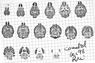
Neuron and glial cell numbers in adult mice While it is satisfying to begin to describe variation in brain weight in terms of individual QTLs, we still do not know what parts of the brain or what cell populations are most and least affected. For example, is there a subset of QTLs that specifically modulate the size of the cerebellum or the numbers of Purkinje cells? We are taking two approaches to answer these types of questions. The first approach is literally to disassemble each brain and map QTLs that control the size of the pieces. Using this approach, we have succeeded in mapping four QTLs that have selective effects of the weight of the cerebellum (Gilissen and Williams 1997; Airey et al. 1998). The second approach is to proceed directly to stereological analyses of individual nuclei and cell types. The main impediment is the stamina that is needed to process and count hundreds of cases. If a single cross could be used to analyze many different CNS structures, and if the genetic resources (genotypes) could be shared, then the effort per QTL might be reduced very substantially. A library of brain tissue from particular crosses would be especially useful because investigators could map multiple QTLs and study the genetic basis of correlations among CNS regions. The mouse brain library. To make this type of analysis practical, Dr. Glenn Rosen (Beth Israel Deaconess Medical Center) and I are in the process of generating an extensive library of sectioned mouse brains suitable for analysis using stereological methods. The current collection is available on the Internet and includes images of approximately 750 brains from 100 strains, all of which were processed in celloidin and cut at 30 µm in either the coronal or the horizontal plane (Fig. 6). The collection contains an average of 6–8 cases from each of the 35 BXD recombinant inbred (RI) strains, the complete set of AXB and BXA RI strains, and most of the common inbred strains listed in Table 1. All sections were stained with cresyl violet, and every 10th section through each brain was mounted on a single slide. Figure 6 is an example of a 1-in-10 series of horizontal sections cut through a 476-mg brain from a 292-day-old male C57BL/6J mouse.
Numbers of neurons and glial cells in the brain of a mouse. Slides such as this can be used for a variety of detailed morphometric studies. For example, the tissue is ideally suited for analysis using either the disector or its close relative—direct three-dimensional counting (Williams and Rakic 1988). Our immediate objective is to uncover QTLs that control total CNS cell number. Estimating the total neuronal and glial population is simple, although in practice it takes about 10 hours. The slide reproduced in Figure 6 was sampled at fixed 2000-µm steps and fields were counted using differential interference contrast optics and a 100X oil-immersion objective (Williams and Rakic 1988; <http://www.nervenet.org/papers/3DCounting.html> for details on methods and implementation). Each sample site, or counting box, had dimensions of 32 by 33 by 20 microns in the X, Y, and Z axes. The final estimate of cell number was based on 175 counts obtained at grid points that intersected tissue. A total of 1908 cells were counted and categorized.It is simple to compute the total cell number of this brain by multiplying the mean cell density by the estimated brain volume obtained by the point count. Each grid point represents a 1.2-mm3 volume of tissue (section interval times section thickness times grid dimensions, or 10 x 30 x 2000 x 2000 µm3). Since 175 sites intersected tissue, the brain volume after processing is ~210 mm3 (24% linear shrinkage based on the fixed brain weight of 476 mg). The brain of this individual contained approximately 75 million neurons, 23 million glial cells, 7 million blood vessel–related endothelial cells, and 3–4 million miscellaneous pial, ependymal, and choroidal cells. Granule cells of the cerebellum made up just under half of the total neuronal population—34 million, a value in close agreement with a previous estimate (Wetts and Herrup 1983). The reliability of the method can be determined easily by an independent count of another slide. It will not be difficult to perform counts like these for all of the BXD strains, and this will make it possible to map QTLs that have specific effects on neuronal and glial cell population size.
Mapping QTLs that modulate neuron number Mapping Cell-Specific QTLs. It is
practical to map QTLs that affect individual neuronal populations. We have
done this type of fine-grained analysis for one of the more accessible
population of neurons in the CNS—the projection neurons of the retina,
also known as retinal ganglion cells (Williams et al. 1998a). One reason
why we chose this population is that it is possible to count these cells
easily and precisely. Each cell has one and only one axon in the optic
nerve, and a quantitative electron microscopic census of axons in a single
cross-section of the nerve provides a reliable and unbiased estimate of
total neuron number (Rice et al. 1996; Williams et al. 1996a). The Nnc1 locus. Using 26 strains of BXD mice, we were able to map the major QTL that is primarily responsible for the bimodality of strain averages (Williams et al. 1998a). There is an excellent correspondence between variation in retinal ganglion cell numbers among these inbred strains and their genotypes on distal chromosome 11. At the Tstap91 locus the correlation reached a peak of 0.69. The genome-wide probability of getting a correlation this high by chance is less than 0.01. We named this QTL neuron number control 1 (Nnc1). Given that only a single neuronal population was studied, this name may seem too broad. Our justification is that we know little about possible pleiotropic effects of this QTL on other neuronal populations. We do know that the QTL is not associated with brain weight in adult mice (the parental strain with the heavier brain has lower ganglion cell number) and it is unlikely that Nnc1 modulates cell populations throughout the CNS. However, preliminary analysis suggests that Nnc1 may have reciprocal effects on cell populations in the inner nuclear layer—the high ganglion cell allele inherited from DBA/2J may actually be associated with low cell numbers in the inner nuclear layer (Williams et al. 1998a,b). Mechanisms of QTL action. A QTL does not need to be cloned before it can be used to study mechanisms of brain development or function. For example, we wanted to determine whether Nnc1 modulates neurogenesis or cell death (Strom and Williams 1998). To answer this question we counted the cell population after neurogenesis, but before the onset of cell death. We were able to show convincingly that the bimodality is produced by a fundamental difference in the total production of retinal ganglion cells. Nnc1 must influence the proliferation of retinal ganglion cells. There are several ways in which Nnc1 could control proliferation: through variation in the progenitor pool size, pathways of cell differentiation, or cell cycle parameters. With such a robust effect and so many strains with alternate phenotypes and alleles, it should now be possible to explore the relative importance of these processes and define more precisely how Nnc1 modulates neurogenesis. Candidate gene analysis. Nnc1
illustrates the power of candidate gene approaches to cloning QTLs.
Nnc1 has been mapped to a 3-cM interval between Hoxb and
Krt1. Remarkably, this short interval which makes up ~0.2% of the
mouse genome includes three superb candidate genes whose products are
expressed in the developing retina and are known to be involved in the
differentiation or proliferation of retinal cells. These candidates are
the retinoic acid alpha receptor (Rara), the thyroid hormone alpha
receptor (Thra), and the ErbB2 receptor (Williams et al.
1998a).
The thyroid hormone receptor is the most tantalizing of the three because
it's natural ligand, thyroxine, is known to modulate the rate and timing
of ganglion cell differentiation in Xenopus laevis during
metamorphosis (Hoskins 1985). Thyroid hormone receptors dimerize with
other members of the steroid hormone receptor family (Piedrafita and Pfahl
1995), and a unique combination of isoforms could explain cellular and
regional specificity of action. The most powerful way to test whether or
not Nnc1 and Thra are one and the same would be to
reciprocally convert high and low strains by swapping the two alleles.
This is a tough experiment, and an expedient intermediary step is to test
effects of targeted deletion of candidate genes. For example, loss of one
candidate gene, Rara, by homologous recombination (Luo et al. 1996)
does not perturb the size of the ganglion cell population (Zhou et al.
1998). In contrast, loss of the Thra gene (Wikström et al. 1998)
has effects on the phenotype that may rival those of Nnc1. Conclusion The quotations taken from the work of Ramón y Cajal and Lashley that introduced this chapter emphasize that the most prominent differences between the brains of mice, chimpanzees, and humans are quantitative; and yet, despite the pride we take in our burgeoning understanding of neuronal development, we have not yet identified a single gene or allele responsible for any part of this astonishing quantitative variation. This is humbling. In our drive to understand the fundamentals of development we can initially be forgiven the blind eye that we have collectively turned to normal variation, but to get beyond descriptions of neuronal development—to get to a second stage of purposeful design, modification, and repair–we will need to understand the subtle, intertwined, and messy molecular genetics that makes a human brain different from that of a mouse and the brain of one human different from that of another (Bartley et al. 1997).
Acknowledgment I thank Dr. Richelle C. Strom for sharing data on the Bsc5 locus. My thanks to Drs. Guomin Zhou, Dan Goldowitz, David C. Airey, and Glenn D. Rosen for their contributions to this work. This research was supported by NINDS RO1 35485.
References Aboitiz F (1996) Does bigger mean better? Evolutionary determinants of brain size and structure. Brain Behav Evol 47:225–245. Adams MD, Soares MB, Kerlavage AR, Fields C, Venter JC (1993) Rapid cDNA sequencing (expressed sequence tags) from a directionally cloned human infant brain cDNA library. Nat Genet 4:373–380. Aiello LC, Wheeler P (1995) The expensive-tissue hypothesis. The brain and the digestive system in human and primate evolution. Curr Anthropol 36:199–221. Airey DC, Strom, RC, Williams RW (1998) Genetic architecture of normal variation in cerebellar size. Soc Neurosci Abst 24:303. Allman JM, McLaughlin T, Hakeem A (1993) Brain weight and life-span in primate species. Proc. Natl. Aca. Sci USA 90:118–122. Armstrong E (1993) Relative brain size and metabolism in mammals. Science 220, 1302–1304. Atchley WR, Riska B, Kohn LAP, Plummer AA, Rutledge JJ (1984) A quantitative genetic analysis of brain and body size associations, their origin and ontogeny: data from mice. Evolution 38:1165–1179. Bartley AJ, Jones DW, Weinberger DR (1997) Genetic variability of human brain size and cortical gyral patterns. Brain 120:257–269. Belknap JK, Phillips TJ, O'Toole LA (1992) Quantitative trait loci associated with brain weight in the BXD/Ty recombinant inbred mouse strains. Brain Res Bull 29:337–344. Belknap JK, Metten P, Helms ML, O'Toole LA, Angeli-Gade S, Crabbe JC, Phillips TJ (1993) Quantitative trait loci (QTL) applications to substances of abuse: physical dependence studies with nitrous oxide and ethanol in BXD mice. Behav Genet 23:213–222. Brockmann GA, Haley CS, Renne U, Knott SA, Schwerin M (1998) Quantitative trait loci affecting body weight and fatness from a mouse line selected for extreme high growth. Genetics 150:369–381. Buck, KJ, Metten P, Belknap JK, Crabbe JC (1997) Quantitative trait loci involved in genetic predisposition to acute alcohol withdrawal in mice. J. Neurosci. 17: 3946–3955. Cheverud JM, Routman EJ, Duarte FAM, van Swinderen B, Cothran K, Perel C (1996) Quantitative trait loci for murine growth. Genetics 142:1305–1319. Churchill GA, Doerge RW (1994) Empirical threshold values for quantitative trait mapping. Genetics 138:963–971. Clark JB, Bates TE, Almeida A, Cullingford T, Warwick J (1994) Energy metabolism in the developing mammalian brain. Biochem Soc Trans 22:980–983. Collins RA (1970) Experimental modification of brain weight and behavior in mice: An enrichment study. Devel Psychobiol 3:145–155. Crabbe JC, Belknap JK, Buck KJ (1994) Genetic animal models of alcohol and drug abuse. Science 264:1715–1723. Crawley JN, Belknap JK, Collins A, Crabbe JC, Frankel W, Henderson N, Hitzemann RJ, Maxson SC, Miner LL, Silva AJ, Wehner JM, Wynshaw-Brois A, Paylor R (1997) Behavioral phenotypes of inbred mouse strains: implications and recommendations for molecular studies. Psychopharmacol 132:107–124. Crusio WE (1992) Quantitative genetics. In: Goldowitz D, Wahlsten D, Wimer RE (eds) Techniques for the genetic analysis of brain and behavior. Elsevier, Amsterdam, pp 231–250. Crusio WE, Schwegler H, van Abeelen JHF (1989) Behavioral responses to novelty and structural variation of hippocampus in mice. I. Quantitative-genetic analysis of behavior in the open field. Behav Brain Res 32:75–80. Dains K, Hitzeman B, Hitzeman R (1996) Genetics, neuroleptic-response and the organization of cholinergic neurons in the mouse striatum. J Pharmacol Exp Therap 279:1430–1438. Darvasi A (1997) Interval-specific congenic strains (ISCS): an experimental design for mapping a QTL into a 1-centimorgan interval. Mamm Gen 8:163–167. Darvasi A (1998) Experimental strategies for the genetic dissection of complex traits in animal models. Nat Genet 18:19–24. DeVoogd TJ, Krebs JR, Healy SD, Purvis A (1993) Relations between song repertoire size and the volume of brain nuclei related to song: comparative evolutionary analyses amongst oscine birds. Proc R Soc Lond B 254:75–82. Dietrich WF, Miller JC, Steen RG, Merchant M, Damron D, Nahf R, Gross A, Joyce DC, Wessel M, Dredge RD, Marquis A, Stein LD, Goodman N, Page DC, Lander ES (1994) A genetic map of the 4,006 simple sequence length polymorphisms. Nat Genet 7:220–245. Eisenberg JF, Wilson DE (1978) Relative brain size and feeding strategies in the chiroptera. Evolution 32:740–751. Eleftheriou BE, Elias MF, Castellano C, Oliverio A (1975) Cortex weight: a genetic analysis in the mouse. J Hered 66:207–212. Festing MFW (1993) Origins and characteristics of inbred strains of mice. Mouse Genome 91:393–509 <http://www.informatics.jax.org/strtools.html>. Flint J, Corley R, DeFries JC, Fulker DW, Gray JA, Miller S, Collins AC (1995) A simple genetic basis for a complex psychological trait in laboratory mice. Science 269:1432–1435. Frankel WN (1995) Taking stock of complex trait genetics in mice. Trends Gen 11:471–477. Fuller JL (1979) Fuller BWS lines: history and results. In: Hahn ME, Jensen C, Dudek BC (eds) Development and evolution of brain size. Academic, New York, pp 187–204. Fuller JL, Wimer RE (1966) Neural, sensory, and motor functions. In: Green EL (ed) The biology of the laboratory mouse, 2nd Ed. Dover, New York, pp 609–628. Fuller JL, Geils HD (1972) Brain growth in mice selected for high and low brain weight. Devel Psychobiol 5:307–318. Fuller JL, Herman BH (1972) Effect of genotype and practice on behavioral development in mice. Devel Psychobiol 7:21–30. Gautvik KM, De Lecea L., Gautvik VT, Danielson PE, Tranque P, Dopazo A, Bloom FE, Sutcliffe JG (1996) Overview of the most prevalent hypothalamus-specific mRNAs, as identified by directional tag PCR subtraction. Proc Natl Acad Sci USA 93:8733–8738. Gilissen E, Zilles K (1996) The calcarine sulcus as an estimate of the total volume of the human striate cortex: A morphometric study of reliability and intersubject variability. J Brain Res 37: 57–66. Gilissen E, Williams RW (1997) Genetic dissection and QTL analysis of forebrain, hindbrain, olfactory bulb, and cerebellum. Soc Neurosci Abst 23:864. Groot PC, Moen CJA, Dietrich W, Stoye JP, Lander ES, Demant P (1992) The recombinant congenic strains for analysis of multigenic traits: genetic composition. FASEB J 6:2826–2835. Hahn ME, Haber SB (1978) A diallel analysis of brain and body weight in male inbred laboratory mice (Mus musculus). Behav Genet 8:251–260. Haley CS, Knott SA (1992) A simple regression method for mapping quantitative trait loci in line crosses using flanking markers. Heredity 69:315-324. Henderson ND (1979) Dominance for large brains in laboratory mice. Behav Genet 9:45–49. Herrup K, Shojaeian-Zanjani H, Panzini L, Sunter K, Mariani J (1996) The numerical matching of source and target populations in the CNS:the inferior olive to Purkinje cell projection. Dev Brain Res 96:28–35. Hitzemann B, Dains K, Kanes S, Hitzemann R (1994) Further studies on the relationship between dopamine cell density and haloperidol-induced catalepsy. J Pharmacol Exp Therap 271:969–976. Hofman MA (1983) Evolution of the brain in neonatal and adult placental mammals: A theoretical approach. J Theoret Biol 105:317–332. Horton JC, Hocking DR (1996) Intrinsic variability of ocular dominance column periodicity in normal macaque monkeys. J Neurosci 16:7228–7339. Hoskins SG (1985) Induction of the ipsilateral retinothalamic projection in Xenopus laevis by thryoxine: results and speculation. J Neurobiol 17:203–229. Jacobs LF, Gaulin SC, Sherry DF, Hoffman GE (1990) Evolution of spatial cognition: sex-specific patterns of spatial behavior predict hippocampal size. Proc Natl Acad Sci USA 87:6349–6352. Johnson TE, DeFries JC, Markel PD (1992) Mapping quantitative trait loci for behavioral traits in the mouse. Behav Genet 22:635–653. Kanes S, Dains K, Cipp L, Gatley J, Hitzemann B, Rasmussen E, Sanderson S. Silverman M, Hitzemann R (1996) Mapping the genes for haloperidol-induced catalepsy. J Pharmacol Exp Ther 277:1016–1025. Katz HB, Davies CA (1983) The separate and combined effects of early undernutrition and environmental complexity at different ages on cerebral measures in rats. Devel Psychobiol 16:47–58. Keverne EB, Martel FL, Nevison CM (1996) Primate brain evolution: Genetic and functional considerations. Proc Roy Soc Lond B 263:689–696. Lande R (1979) Quantitative genetic analysis of multivariate evolution, applied to brain:body size allometry. Evolution 33:234–251. Lander ES, Botstein D (1989) Mapping Mendelian factors underlying quantitative traits using RFLP linkage maps. Genetics 121:185–199. Lander E, Kruglyak L (1997) Genetic dissection of complex traits: guidelines for interpreting and reporting linkage results. Nat Genet 11:241–247. Lander ES, Schork NJ (1994) Genetic dissection of complex traits. Science 265:2037–2048. Lashley KS (1949) Persistent problems in the evolution of mind. Quart Rev Biol 24:28–42. Le Roy I, Perex-Diaz F, Cherfouh A, Roubertoux PL (1999) Preweanling sensorial and motor development in laboratory mice: quantitative trait loci mapping. Devel Psychobiol 34: in press. Lewontin RC (1957) The adaptations of populations to varying environments. Cold Spring Harbor Sympos Quart Biol 22:395–408. Lipp HP (1989) Non-mental aspects of encephalization: the forebrain as a playground of mammalian evolution. Hum Evol 4:45–53. Lipp HP, Schwegler H, Crusio WE, Wolfer DP, Leisinger-Trigona MC, Heimrich B, Driscoll P (1989) Using genetically-defined rodent strains for the identification of hippocampal traits relevant for two-way avoidance behavior: a non-invasive approach. Experientia 45:845–859. Lu L, Airey DC, Williams RW (2000) Genetic architecture of the mouse hipocampus: identification of gene loci with specific effects on hippocampal size. in submission. Luo J, Sucove HM, Bader JA, Evans RM, Giguere V (1996) Compound mutants for retinoic acid receptor (RAR) beta and RAR alpha 1 reveal developmental functions of multiple RAR beta isoforms. Mech Dev 55:33–44. Lynch M, Walsh B (1998) Genetics and analysis of quantitative traits. Sinauer, San Francisco. Manly KF, Olson JM (1999) Overview of QTL mapping software and introduction to Map Manager QT. Mammalian Genome, 10:327–334. Martin RD (1981) Relative brain size and metabolic rate in terrestrial vertebrates. Nature 293:57–60. Pagel MD, Havey PH (1990) Diversity in the brain sizes of newborn mammals: allometry, energetics, or life history tactics? Bioscience 40:116–122. Pakkenberg B, Gundersen HJG (1997) Neocortical neuron number in humans: effect of sex and age. J Comp Neurol 384:312–320. Piedrafita FJ, Pfahl M (1995) Thyroid hormone receptors. In: Baeuerle PA (ed) Inducible gene expression, Vol 2. Birkhäuser, Boston, pp 157–185. Plomin R, McClearn GE (1993) Quantitative trait loci (QTL) analyses and alcohol-related behaviors. Behav Genet 23:197–211. Plomin R, McClearn GE, Gora-Maslak G, Neiderhiser JM (1991) Use of recombinant inbred strains to detect quantitative trait loci associated with behavior. Behav Genet 21: 99–116. Ramón y Cajal S (1890) Estudios sobre la corteza cerebral humana. III. Cortez motriz. Revista trimestral micrográfica 5:1–11. [Trans by Jacobson M (1991) In: Developmental neurobiology, 3rd Ed. Plenum, New York, p 401]. Rensch B (1956) Increase of learning capability with increase of brain-size. Amer Natur 90:81–95. Rice DS, Williams RW, Goldowitz D (1995a) Genetic control of retinal projections in inbred strains of albino mice. J Comp Neurol 354:459–469. Rise ML, Frankel WN, Coffing JM, Seyfried TN (1991) Genes for epilepsy mapping in the mouse. Science 253:669–673. Roderick TH (1979) Genetic techniques as tools of analysis of brain-behavior relationships. In: Hahn ME, Jensen C, Dudek BC (eds) Development and evolution of brain size. Academic, New York, pp 133–145. Roderick TH, Wimer RE, Wimer CC, Schwartzkroin PA (1973) Genetic and phenotypic variation in weight of brain and spinal cord between inbred strains of mice. Brain Res 64:345–353. Roderick TH, Wimer RE, Wimer CC (1976) Genetic manipulation of neuroanatomical traits. In: Petrinovich L, McGaugh L (eds) Knowing, thinking, and believing. Plenum, New York, pp 143–178. Roff DA (1997) Evolutionary quantitative genetics. Chapman Hall, New York. Sacher GA, Staffeldt EF (1974) Relation of gestation time to brain weight for placental mammals: implication for the theory of vertebrate growth. Amer Natur 108:593–615. Schwegler H, Lipp HP (1983) Hereditary covariations of neuronal circuitry and behavior: correlations between the proportions of hippocampal synaptic fields in regioi inferior and two-way avoidance in mice and rats. Behav Brain Res 7:297–305. Seyfried TN, Daniel WL (1977) Inheritance of brain weight in two strains of mice. J Hered 68:337–338. Seyfried TM, Glaser GH, Yu RK (1979) Genetic variability for regional brain gangliosides in five strains of young mice. Biochem Genet 17:43–55. Sprott RL, Staats J (1981) Behavioral studies using genetically defined mice–a bibliography. Behav Genet 11:73–84. Stensaas SS, Donald MA, Eddington DK, Dobelle WH (1974) The topography and variability of the primary visual cortex in man. J Neurosurg 40:747–755. Storer JB (1967) Relation of lifespan to brain weight, body weight, and metabolic rate among inbred mouse strains. Exp Geront 2:173–182. Strom RC (1999) Genetic control of neuron number. Dissertation, Univ Tenn, Memphis. Strom RC, Williams RW (1997) Mapping genes that control variation in brain weight using F2 intercross progeny. Soc Neurosci Abst 23:864. Strom RC, Williams RW (1998) Cell production and cell death in the generation of variation in neuron number. J Neurosci 18:9948–9953. Sutcliffe JG (1988) mRNA in the mammalian central nervous system. Annu Rev Neurosci 11:157–198. Takahashi JS, Pinto LH, Vitaterna MH (1994) Forward and reverse genetic approaches to behavior in the mouse. Science 1724:1724–1733. Tanksley SD (1993) Mapping polygenes. Annu Rev Genet 27:205–233. Taylor BA (1978) Recombinant inbred strains. Use in gene mapping. In: Morse H (ed) Origins of inbred mice. Academic, New York, pp 423–438. Toth L.A., Williams, R. W. (1988). Genetic analysis of complex quantitative traits using inbred mice. Sleep Res Soc Bull 4:50–56. Usui H, Falk JD, Dopazo A, de Lecea L, Erlander MG, Sutcliffe JG (1994) Isolation of clones of rat striatum-specific mRNAs by directional tag PCR subtraction. J Neurosci 14:4915–4926. Vadasz C, Sziraki I, Sasvari M, Kabai P, Murthy LR, Saito M, Laszlovszky I (1998) Analysis of the mesotelencephalic dopamine system by quantitative-trait locus introgression. Neurochem Res 23:1337–1354. Wahlsten D (1975) Genetic variation in the development of mouse brain and behavior: evidence from the middle postnatal period. Develop Psychobiol 8:371–380. Wahlsten D (1983) Maternal effects on mouse brain weight. Devel Brain Res 9:216–221. Wahlsten D (1992) The problem of test reliability in genetic studies of brain-behavior correlation. In: Goldowitz D, Wahlsten D, Wimer RE (eds) Techniques for the genetic analysis of brain and behavior: focus on the mouse. Elsevier, Amsterdam, pp 407–422. Wahlsten D (1994) The intelligence of heritability. Can Psych 35:244–267. Ward BC, Nordeen EJ, Nordeen KW (1998) Individual variation in neuron number predicts differences in the propensity for avian vocal imitation. Proc Natl Acad Sci USA 95:1277–1282. Wetts R, Herrup K (1983) Direct correlation between Purkinje and granule cell number in the cerebella of lurcher chimeras and wild-type mice. Dev Brain Res 10: 41–47. Wikström L, Johansson C, Saltó C, Barlow C, Campos Barros A, Baas F, Forrest D, Thorén P, Vennström B (1998) Abnormal heart rate and body temperature in mice lacking thyroid hormone receptor 1. EMBO J 17:455–461. Williams RW (1998) Neuroscience meets quantitative genetics: Using morphometric data to map genes that modulate CNS architecture. In: Morrison J, Hof P (eds) Short course in quantitative neuroanatomy. Society of Neuroscience, Washington DC, pp 66–78. Williams RW, Herrup K (1988) The control of neuron number. Annu Rev Neurosci 11:423–453. Williams RW, Rakic P (1988) Three–dimensional counting: An accurate and direct method to estimate numbers of cells in sectioned material. J Comp Neurol 278:344–352. Williams RW, Zhou G (1999) Genetic control of eye size: A novel quantitative genetic approach. Invest. Ophthalmol Vis Sci Suppl 40:SXXX. Williams RW, Cavada C, Reinoso-Suárez F (1993) Rapid evolution of the visual system: a cellular assay of the retina and dorsal lateral geniculate nucleus of the Spanish wildcat and the domestic cat. J Neurosci 13:208–228. Williams RW, Strom RC, Rice DS, Goldowitz D (1996a) Genetic and environmental control of variation in retinal ganglion cells number in mice. J Neurosci 16:7193–7205. Williams RW, Strom RC, Goldowitz D (1996b) Mapping quantitative trait loci that control normal variation in brain weight in the mouse. Soc Neurosci Abst 22: 518. Williams RW, Goldowitz DG, Strom RC (1997) Brain weight in relation to body weight, age, and sex: A multiple regression analysis. Soc Neurosci Abst 23:864. Williams RW, Strom RC, Goldowitz D (1998a) Natural variation in neuron number in mice is linked to a major quantitative trait locus on Chr 11. J Neurosci 18:138–146. [Williams RW, Airey DC, Kulkarni A, Zhou G, Lu L (2000) Neurogenetic analysis of olfactory bulbs in mice: QTLs on chromosomes 4, 6, 11, and 17 modulate growth.Behavior Genetics, in press.] Williams RW, Strom RC, Zhou G, Yan Z (1998b) Genetic dissection of retinal development.Sem Cell Devel Biol 9:249–255. Wimer C (1979) Correlates of mouse brain weight: A search for component morphological traits. In: Hahn ME, Jensen C, Dudek BC (eds) Development and evolution of brain size. Academic, New York, pp 147–162. Wimer C, Prater L (1966) Behavioral differences in mice genetically selected for high and low brain weight. Psychol Rep 19:675–681. Wimer RE, Wimer CC (1985) Animal behavior genetics: a search for the biological foundation of behavior. Annu Rev Psychol 36:171–218. Wimer RE, Wimer CC (1989) On the sources of strain and sex differences in granule cell number in the dentate area of house mice. Dev Brain Res 48:167–176. Wimer RE, Wimer CC, Roderick TH (1969) Genetic variability in forebrain structures between inbred strains of mice. Brain Res 16:257–264. Wimer RE, Wimer CC, Vaughn JE, Barber RP, Balvanz BZ, Chernow CR (1978) The genetic organization of neuron number in the area dentata of mouse mice. Brain Res 157:105–122. Wright S (1978) Evolution and the genetics of populations, Vol 4. Variability within and among natural populations. U Chicago, Chicago. Zamenhof S, van Marthens E (1976) Neonatal and adult brain parameters in mice selected for adult brain weight. Dev Psychobiol 9:587–593. Zamenhof S, van Martens E, Gauel L (1971) DNA (cell number) in neonatal brain: second generation (F2) alternation by maternal (F0) dietary protein restriction. Science 172:850–851. Zhou G, Williams RW (1999a) Mouse models for the analysis of myopia: an analysis of variation in eye size of adult mice. Optom Vis Sci, in press. Zhou G, Williams RW (1999b) Eye1 and Eye2: Gene loci that modulate eye size, lens weight, and retinal area in mouse. Invest Ophthalmol Vis Sci 40:817–825. Zhou G, Strom RC, Giguere V, Williams RW (1998) Modulation of retinal cell populations and eye size in retinoic acid receptor knockout mice. Soc Neurosci Abst 24:1033.
Since 23 March 1999
|
||||||||||||||||||||||||||||||||||||||||||||||||||||||||||||||||||||||||||||||||||||||||||||||||||||||||||||||||||||||||||||||||||||||||||||||||||||||||||||||||||||||||||||||||||||||||||||||||||||||||||||||||||||||||||||||||||||||||||||||||||||||||||||||||||||||||||||||||||||||||||||||||||||||||||||||||||||||||||||||||||||||||||||||||||||||||||||||||||||||||||||||||||||||||||||||||||||||||||||||||||||||||||||||||||||||||||||||||||||||||||||||||||||||||||||||||||||||||||||||||||||||||||||||||||||||||||||||||||||||||||||||||||||||||||||||||||||||||||||||

Neurogenetics at University of Tennessee Health Science Center
| Print Friendly | Top of Page |
Mouse Brain Library | Related Sites | Complextrait.org
