New figures, text, and links have been incorporated into the revision. Revised HTML (http://www.nervenet.org/netpapers/Rosen/Cav90/Caval.html) copyright ©1999 by Glenn D. Rosen

While the Cavalieri approach provides a better approximation of volume under some circumstances, it requires equally-spaced sections. We therefore describe methods for the estimation of brain volume from unequally-spaced sections, including an estimator based on the fitting of piece-wise parabolic curves to the data. We outline a series of guidelines for the use of these mathematical rules in the estimation of brain volume from serial sections.

Currently, estimating brain volume by analyzing parallel, systematically sampled serial sections through the material is the most common technique (2, 3, 5, 6). A calculation of volume involves essentially the numerical integration of a curve that plots area against the appropriate x, y, or z coordinate (i.e., the coordinate orthogonal to the plane of section). Numerical integration is typically performed using either Cavalieri’s rule (7), a trapezoidal (3, 6) or parabolic (Simpson’s or Durand’s) (2, 4) rule. From a mathematical perspective, Cavalieri’s rule is an unbiased estimator based on the rectangular approximation of the area under a curve (8, 9), the trapezoidal approximation further enhances this rectangular approximation, and the parabolic approach is an improvement over the trapezoidal, with Simpson’s rule being the preferred implementation (10). Some workers have argued strongly for the parabolic approximation (11) while others have supported the use of Cavalieri’s rule, claiming its efficiency for volume estimation, especially for irregular brain regions (7). Given that these calculations are now almost always performed on a computer, the differences in computational effort among Cavalieri’s, the trapezoidal, and parabolic estimations of volume are insignificant. It seems reasonable, therefore, to opt always for the most accurate of the three methods.

There are, however, practical differences between the methods. Simpson’s rule requires an odd number of cross-sectional area measurements at equally spaced intervals through the brain (10), and while “Simpson’s three-eighths” or Durand’s rule will work on odd or even numbers of sections, it also requires equal spacing (10, 12). Cavalieri’s rule also requires equal spacing of points (8, 9). These are conditions not always possible to meet in brain histology as some sections from a series are not well suited (because of reasons of cutting or staining artifact, for example) for morphometric measurement. This begs the question of whether the various computational approaches are equivalent in the more demanding setting of real brain measurements of volume.

Our goal, then, was to make a real-world comparison of these techniques as they apply to brain morphometry in an effort to establish practical and useful guidelines for their use. Using both idealized (i.e., mathematically contrived) data and morphometric measures from actual brain material, these methods were directly tested against one another. In addition, we describe a more general mathematical treatment of piece-wise parabolic integration which relaxes the equi-spaced requirement of the traditional parabolic rule. Such a formulation permits greater flexibility in sectioning protocols, but has its own idiosyncratic problems which cannot be ignored.

METHODS

In order to test these rules, we performed the following tests: (1) We compared the accuracy of results computed from systematic sampling of two mathematically simulated brain regions of known volume using the parabolic, trapezoidal, Cavalieri, and rectangular estimators. (2) We measured one regularly-shaped , and one irregularly-shaped simulated brain region. In addition, we examined the effect of increase of sampling distance on the accuracy of these estimations. (3) We randomly “lost” sections from the samples and determined which of the rectangular, trapezoidal, and piece-wise parabolic estimators were best on unequally spaced sections. (4) Finally, we estimated volume of the visual cortex (a regularly-shaped region) and the caudate nucleus (an irregularly-shaped region) of the rat.

After a brief discussion of sampling protocols, we catalog the equations that can be used to compute volume from serial cross-section area measurements. Most of these can be found readily in other sources and are included here for completeness. Some additional mathematical detail is provided for the description of the parabolic calculations that permit unequally spaced sections. Finally, we describe how these various methods were applied to the mathematically simulated brain regions.

Sampling Protocols

In the estimation of brain volume from serial sections, one basic presumption is that not every section is to be analyzed; usually every fifth or tenth section is used. There are basically two possibilities for the selecting sections for use in the analysis—“non-systematic” and “systematic” sampling—and the choice between these is critical in determining the proper volume estimator. A non-systematic sample is obtained by looking through all the sections to find the very first one in which the structure of interest appears. That section, and all subsequent sections that are the desired distance apart, is analyzed until the structure of interest no longer appears. The systematic sampling paradigm, in practice, involves the analysis of an equally-spaced series of sections beginning with the first section on which the region appears in a randomly chosen series, and continuing for each section of the series that contains the structure. Thus, in the systematic approach the first section analyzed may or may not be the first section on which the region of interest appears. In this paper, we focus on analysis using systematic sampling.

Rectangular Estimation of Morphometric Volume

The rectangular estimate of morphometric volume for equally spaced sections (V_Requal) is determined by the following formula:

where “d” = distance between the sections that are being analyzed (not to be confused with the section thickness “t”), “y_i” = cross sectional area of the ith section through the morphometric region, and “n” = total number of sections (8).

For unequal spacing, the rectangular estimation of morphometric volume (V_Runequal) is defined in Equation 2

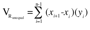where “x_i” = the distance orthogonal to the plane of section of the ith section (usually section number multiplied by section thickness).

The rectangular approach, as others have pointed out (7), is appropriate only for non-systematic sampling. For systematic sampling, the rectangular method is incorrect and Cavalieri’s estimate or the “basic volume estimator” (see below) should be used. We include the rectangular approach in our analysis as an empirical illustration of the potential problems of using this approach with the systematic sampling procedure.

Cavalieri’s Estimator of Morphometric Volume

Cavalieri’s estimator of volume (V_C) is a statistically unbiased form of the rectangular approach which requires systematic sampling (Equation 3):

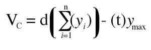where “y_MAX” is the maximum value of “y” and “t” = section thickness. Their product is subtracted from the basic equation as a correction for overprojection (8)

Trapezoidal Estimation of Morphometric Volume

The trapezoidal estimate of morphometric volume for equally spaced sections (V_Tequal) is determined by the following formula (10):

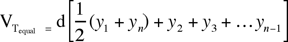For unequal spacing between sections, the trapezoidal estimate of morphometric volume (V_Tunequal) becomes:

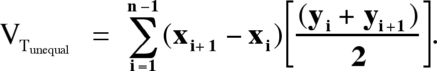Parabolic Estimation of Morphometric Volume

The Simpson’s rule formulation for the determination of area under a curve (V_S) found in numerical analysis texts is a closed form (i.e., exact) simplification of the area under a series of parabolas (10):

where total number of sections (“n”) is required to be odd.

One can estimate the area under a curve with an even number of sections using either a modification of “Simpson’s three-eighths” rule (V_S3/8; [12])

or Durand’s (V_D) equation (10):

Of these two rules, the former (V_S3/8) is more accurate.

To relax the need for equal spacing requires a slightly more general approach to the problem of fitting parabolas in a piece-wise fashion to the data points. The equation of a parabola is:

where “a,” “b,” and “c” are constants. From simple geometry, it is clear that there is exactly one parabola that passes through three points in a plane. Finding that parabola is not a curve fit in the usual “least squares” sense of that term. It is possible to compute exactly the “a,” “b,” and “c” of the parabola that will pass through the points. More than one method is available to do this (13), but perhaps the easiest to follow is shown here.

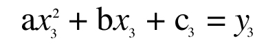
Treat “a,” “b,” and “c” as unknowns and write three equations that must be true in order for the parabola to pass through the three known points (x₁,y₁), (x₂,y₂), (x₃,y₃):

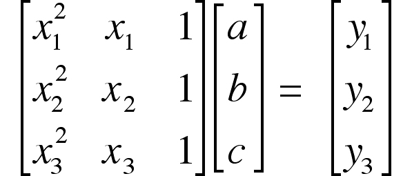
This is a set of three simultaneous equations for the three unknowns “a,” “b,” and “c”. Writing the equations in matrix form,

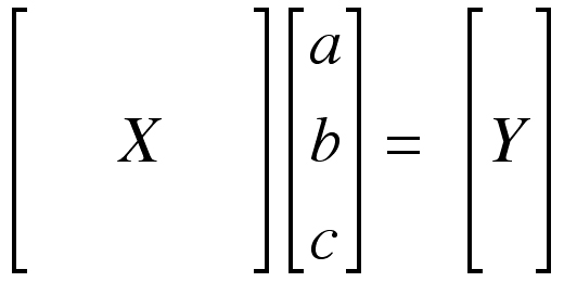
or

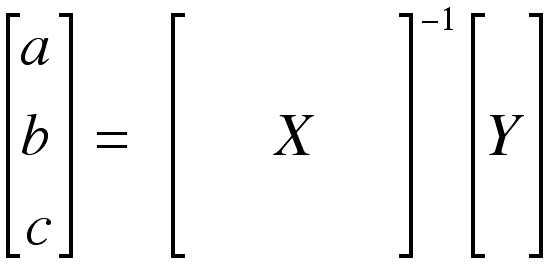
The unknowns “a,” “b,” and “c” can be found by multiplying the matrix Y by the inverse of the matrix X (X^-1).

This operation is easily implemented on a computer. It is important to see that no assumption on the spacing of the data is made in this analysis.

Once the equation of the parabola has been found for these three data points, the area under the parabola (which is equivalent to the brain volume in the current instance) is computed by integrating:

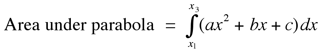In the case of estimating brain volume from cross-sectional area measurements, there will almost certainly be more than three data points available. The extension of the equations above to this situation is straightforward. Simply divide the data into groups of three points, (x₁, x₂, x₃), (x₃, x₄, x₅), and so on, and perform the calculation of “a,” “b,” and “c” on each group independently. The total area under the curve specified by the data (V_P) would be:

where the subscripts on “a,” “b,” and “c” denote the parabola parameters computed from the different groups of data points, “x” = the distance orthogonal to the plane of section (usually section number times section thickness), and “n” = total number of sections.

Performing the integrations analytically, the expression above becomes:

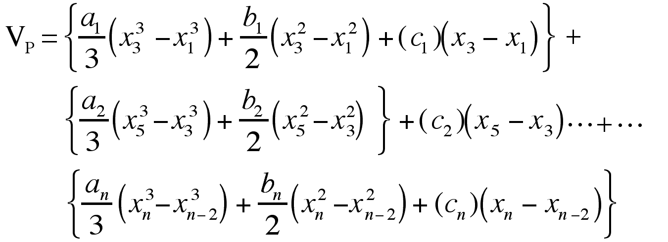As with Simpson’s rule, there must be an odd number of sections studied for these equations to work without modification. It should be noted that in the case of equi-spaced odd sections, V_P = V_S. In the instances where there are even numbers of sections, the area under the curve of the last two sections can be estimated using the trapezoid rule.

Mathematically Simulated Brain Regions

To simulate mathematically a set of measurements from regular (i.e., with cross-sectional areas symmetric about the midline of the axis orthogonal to the plane of section) brain sections, the cross sectional area of each section was computed using the following formula:

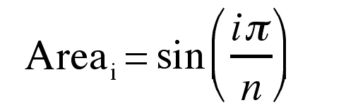where “n” is the total number of sections in the simulated brain and “i” is the section number. This equation produces the top half of a sine-wave (Figure 1). This simulated brain shape was chosen because it is a reasonable representation of cross-section area variations in some brain regions (e.g., architectonic regions of neocortex).

Figure 1. Line plot of cross-sectional area vs. section number for the four experimental groups. For mathematically simulated regularly- and irregularly-shaped, curves are continuous functions shown here with a 25 section sampling frequency. To convert section number to distance (in mm), multiply by the section thickness (Mathematically simulated = 0.035 mm, Caudate Nucleus and Visual cortex = 0.030 mm). See text for explanation.

To simulate mathematically a set of measurements from irregular (i.e., with cross-sectional areas asymmetric about the midline of the axis orthogonal to the plane of section) brain sections, the cross sectional area of each section was computed using the following formula:

Equation 20

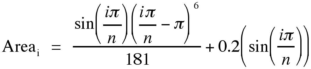where “n” is the total number of sections in the simulated brain and “i” is the section number (Figure 1). Division by 181 normalizes the curve so that its maximum is “1”, as is the case for the curve generated by Equation 19. This irregular curve is a reasonable representation of cross-section area variations in some brain regions (e.g., fascia dentata; (7, 8).

Morphometric Measures

The caudate nucleus and the visual cortex of 19 rats were traced in a series of every tenth section in both the right and left hemispheres using a camera lucida attachment to a Zeiss Universal microscope at a magnification factor ranging from 30–33X. The cross section areas of the tracings were obtained using a Zeiss MOP-3 planimeter. The total number of sections in which the caudate nucleus appeared ranged from 12–19, with the visual cortex appearing in 9–16 sections.

Experimental Protocol

All calculations were performed on a Macintosh® IIcx (Apple Computer, Cupertino, CA) using Microsoft Excel® (Microsoft Corporation, Redmond, WA), a spreadsheet program (templates available online as a Macintosh .hqx file, a UUencoded file. or by email request). All estimations (Cavalieri, rectangular, parabolic, and trapezoidal) were computed concurrently.

Mathematical Simulation of Brain Volume in Equally-Spaced Sections

The same region from ten “brains” was simulated for the comparison. Each had a different anterior-posterior dimension and, since section thickness was a constant, each had a different number of “sections” for which simulated data was available. Section thickness for both the regularly- and irregularly-shaped brains was set arbitrarily at 35 µm (see Figure 1). The smallest simulated region had 411 sections, and that number was increased by 10 for each subsequent region so that the largest had 501 sections — the between-brain variability was therefore ±10%. Of all the computed sections, only a small subset of systematically sampled sections was used in the calculation of volume, thereby replicating the usual situation when analyzing real brain material.

To assess how sensitive the volume estimations were to the number of sections used in the analysis, we computed total brain volume based on sampling at 0.35 mm intervals (every 10th section; 40-50 total sections sampled), 0.70 mm (every 20th: 20-25 sections), 1.4 mm (every 40th; 10-13 sections), or 2.8 mm (every 80th; 5-7 sections). The starting section was chosen randomly from a range defined between the first section and the distance between sampled sections. Thus, for the case of the 0.35 mm distance, the starting section was randomly chosen between 1 and 10 inclusive. This satisfies the criteria of systematic sampling, and accurately simulates the way in which serial sections are chosen for analysis in actual brain material. These volume estimates were compared to the actual volume that could be computed by analytically integrating the two functions. Values within the 50% confidence limits of the actual values were deemed to be acceptably accurate.

Mathematical Simulation of Brain Volume in Unequally-Spaced Sections

The same region from the ten “brains” described above was used in the calculation of volume. To simulate the case where sections are lost to suboptimal histology, from 1-3 sections were randomly removed from those chosen to be analyzed. The volume of the regions was then estimated using the rectangular, trapezoidal and piece-wise parabolic equations and the results compared to the actual volume that could be computed by analytically integrating the two functions. Values within the 50% confidence limits of the actual values were deemed to be acceptably accurate.

Caudate Nucleus and Visual Cortex Measures

The measure of volume of visual cortex (area 17 of Krieg (14, 15) , area OC1 of Zilles (16) and of the caudate nucleus was undertaken on the brains of nineteen 120 day old rats whose brains, acquired for another experiment, were embedded in celloidin and cut coronally at 30 or 40 µm (See Figure 1). The volumes for the left and right cortices were computed separately and then summed for the final value reported.

RESULTS

Regularly-shaped, equally-spaced brain regions

The true value and the estimation of the area of the regular, simulated brain region using each of the estimators are summarized in Figure 2. All values for the Cavalieri estimation fell within the 50% confidence limits of the population mean. Using the parabolic rules, all fell within this same confidence limit with the exception of the estimate based on sampling every 80th section. The rectangular and trapezoidal estimates fell outside of these confidence limits when the sampling frequency fell below 10-13 sections.

Irregularly-shaped, equally-spaced brain regions

The results for the estimation of volume from irregular, mathematically simulated brain regions are summarized in Figure 2. As with the case with the regularly-shaped brain regions, the estimates based on the Cavalieri approach fell within the 50% confidence limits for all sampling distances. The parabolic estimators were accurate only when the number of sections sampled was 20-25 or greater, while the trapezoidal estimations were inaccurate for all but the most frequent section-sampling frequency. The rectangular estimation was accurate when the number of sections was 10-13 or greater.

Figure 2. Mean ± S.E.M. for rectangular (solid bars), Cavalieri (hatched bars), trapezoid (open bars), and parabolic (grey bars) estimations of volume in mathematically simulated regularly-shaped and irregularly-shaped brain regions with equal spacing between sections. Results are shown from estimates based on four different distances between the sections. The mean and S.E.M. are computed from sampling 10 simulated brain regions at varying section numbers. The solid line is the true population mean value, and the shaded area on either side of this line represent the 50% confidence limits of the mean.

Regularly-shaped, unequally spaced brain regions

The true value and the estimation of this area using each of the estimators are summarized in Figure 3. All three estimations were accurate only when at least 20–25 sections were sampled, with no obvious advantage of one approach over the other.

Figure 3. Mean ± S.E.M. for rectangular (solid bars), Cavalieri (hatched bars), trapezoid (open bars), and parabolic (grey bars) estimations of volume in mathematically simulated regularly-shaped and irregularly-shaped brain regions with unequal spacing between sections, with 1–3 sections randomly removed from the analysis. Results are shown from estimates based on four different distances between the sections. . The mean and S.E.M. are computed from sampling 10 simulated brain regions at varying section numbers. The solid line is the true population mean value, and the shaded area on either side of this line represent the 50% confidence limits of the mean.

Irregularly-shaped, equally spaced brain regions

The results for the estimation of volume from irregular, mathematically simulated brain regions are summarized in Figure 4. Estimations based on 40-50 sections were accurate with any of the methods, however, none were accurate at any section sampling frequency below that

Figure 4. Mean ± S.E.M. for rectangular (solid bars), trapezoidal (open bars), and parabolic (grey bars) estimations of volume in visual cortex and the caudate nucleus brain regions. These number are the sum of volume estimations derived seperately from the left and right hemispheres. The shaded areas represent the 50% confidence limits of the mean of the Cavalieri estimation, the solid line is the mean value. N = 19 for both groups.

Actual Morphometric Measures. Because there is no actual value for these measures (the volumes of the real brain regions are not known a priori), the means from the estimators were compared against that derived from the Cavalieri estimation as it proved to be the most accurate measure in the mathematically simulated brain regions. There were no significant differences among the four volume estimators for either the caudate nucleus or visual cortex measures.

DISCUSSION

Mathematically Simulated Brain Regions - Equal Spacing

Previous reports have suggested that there is no significant difference between parabolic and trapezoidal estimation of brain volume from serial sections (7). These authors further contend that the use of Cavalieri’s rule allows for accurate volume estimation using relatively few sections, and are therefore more efficient (8, 9). Our estimations based on mathematical simulations of brain regions unequivocally support this theoretical contention. This is true for both regularly- and irregularly-shaped regions. In contrast, parabolic estimators, which are mathematically superior for estimating area under a curve, are not efficient when subjected to the conditions of systematic sampling. The rectangular estimation, as discussed above, is not appropriate for systematic sampling and is noticably inaccurate when compared to the Cavalieri estimate, especially when used with few sections.

Estimations from unequally-spaced sections

Our analysis shows that while it is possible to estimate volume from systematic serial sections using a rectangular, trapezoidal, and piece-wise parabolic approach, these methods are only accurate in regularly-shaped brain regions when a relatively large number of sections are counted. If one accepts the admittedly conservative criteria of having the estimates lying within the 50% confidence limits, then one needs to sample at least 20-25 sections in order to achieve an accurate estimate. Using a less stringent 95% criteria, one need sample only 10-13 sections. Estimations of irregularly-shaped brain regions with section missing, on the other hand, are inaccurate using either criteria at that section sampling frequency—on needs at least 20–25 for a 95% and over 40 for a 50%.

Morphometric Measures from Actual Brain Regions

Unlike the case with the mathematically-simulated brain regions, the estimations from actual morphometric measures have no true population mean so it is theoretically impossible to determine which of the several methods of volume estimation is most accurate. It is therefore more reasonable to determine whether the methods differ significantly in their estimates. We found no differences between regional volumes computed using any of the rules for the estimate of caudate nucleus or visual cortex volume, with the percentile differences being less than 1% for the former and less than 1.5% for the latter.

Guidelines

We therefore suggest the following guidelines for the estimation of volume from serial sections in regularly- or irregularly-shaped brain regions, keeping in mind that estimations based on actual morphometric measures yielded very similar results with all four of the methods used

We suggest use of Cavalieri’s rule in virtually every equally-spaced case. In circumstances where many sections are available for analysis, it provides numbers very similar to the other methods. When few sections are available, it provides the best estimate of volume.

For unequally spaced sections, any of the methods described is appropriate but only when relatively large numbers of sections are sampled.

ACKNOWLEDGMENTS

This work was supported, in part, by NIH grant 20806, the Orton Dyslexia Society, and the Carl J. Herzog Foundation. The authors wish to thank Dr. Albert Galaburda for his comments on an earlier version of the manuscript and the referees for their helpful comments on an earlier version of the manscript.

Footnotes

In the current report, the histological problems associated with the accurate measurement of brain volume (e.g., accurate determination of section thickness, anatomic parcellation, etc.) are not discussed. The reader is referred to (7) for a complete discussion of these issues. We focus instead on comparing the available computational techniques. (back to text)

Regularly shaped brains regions are defined as those regions with cross-sectional areas symmetric about the midline of the axis orthogonal to the plane of section, and irregularly-shaped regions as those with cross-sectional areas asymmetrical about the midline of this axis. (back to text)